Statistics and data analysis

Antoine Géré

General informations

Organization

	S2	S3	S4	S5
Lectures	8 (12h)	8 (12h)	8 (12h)	8 (12h)
Tutorials	8 (12h)	8 (12h)	8 (12h)	8 (12h)
tot.	16 (24h)	16 (24h)	16 (24h)	16 (24h)

• Lectures : no need to bring your personal computer
• Tutorials : bring your personal computer

https://ant0in3g.github.io/sTa7.html \(\to\) look at your stickers !

Evaluations and Group projets

Evaluations

For each semester :

• One mid-semester exam (1h30)
• One final exam (1h30)

Group projets

• Semester 2 :

  Première Analyse en Statistique Descriptive (PASD)

• Semester 4 :

  Première Expérience en Analyse de Données (PEAD)

• Semester 6 :

  Projet d’Initiation à la Démarche Expérimentale (PIDEx)

Resources and OneDrive folder

Resources

• Slides du cours

• Cours complet de Statistiques et analyse de données (en construction)

• Travaux dirigés

• Sujets d’examens corrigées des années passées

• An Introduction to Statistical Learning from the Stanford University with a YouTube playlist of the lectures

Shared OneDrive folder

A OneDrive folder has been shared with every student

To Do !

Synchornize this folder on your laptop OR create a shortcut on your own OneDrvive

Introduction to statistics and/with R

• Data : interesting

\(\to\) they help us understand the world !

• Statistics : fundamental in science

\(\to\) needed in the design, analysis, and interpretation of experiments !

A brief intro to R and RStudio

• Free open source language
• Built to do statistics
• Updated by the mathematician from all over the world
• Amazing graphics !
• Widely used in biology, agronomy, economy, …

R and RStudio

Learn it, love it, use it !

Installation of R and RStudio

To Do !

Install R and RStudio for next class !

Basics of R and RStudio

A very great video to learn the basics of R

Good habits

• create a project on RStudio
• create ALWAYS 4 folders :
  • data_raw
  • data
  • img
  • doc
• Use the help function ! … and also chat GPT …
  WARNING ! It often writes code wayyyy too complicated !
• What you see in your OneDrive folder :

Launch RStudio

Always launch your RStudio project with

Using RStudio

Import DATA into RStudio

• Data used for this class : Data.Lecture.xlsx

Important

You can download it by clicking on Data.Lecture.xlsx !

• Import data from an excel file

library(readxl)
my.data <- read_excel("data_raw/Data.Lecture.xlsx")

• Possible to import data from many more file formats …

Let’s get started

NOW “doing statistics” can get started !

Exploring data

Def.

• A variable \(X\) is any characteristic observed in a study.
• The data values that we observe for a variable are called observations

Qualitative / Categorical Variable

A variable is called qualitative if each observation belongs to a set of distinct categories

• Nominal : Categories are disconnected. (Examples : Hair Color, Animal Species, …)

• Ordinal : Categories are ranked (Example : Level of Education, …)

Quantitative / Numerical Variable

A variable is called quantitative if observations on it take numerical values that represent different magnitudes of the variable

• Discrete : the variable assume values in a countable set (Examples : Number of episode in a series, Grades, …)

• Continuous : the variable assume values in a continuous set (Examples : Time, most physical measurements, …)

In a dataset (sample of a population) we have measurements of variables for different individuals.

• Unit / individual : A member of a population
• Population : The collection of all individuals / units that we want to know more about
• Sample : The subset of the population we observe
• Modality : The distinct values or categories that the variable can take

Before making advanced statistics with our data it is essential to examine all our variables !

Why ? To “listen” to the data :

• to catch mistakes
• to see patterns in the data
• to find violations of statistical assumptions
• to generate hypotheses
• … and because if you don’t, you will have trouble later !

• We will recall notions of descriptive Statistics with R
  
• This has been written using this webpage (INRAE)

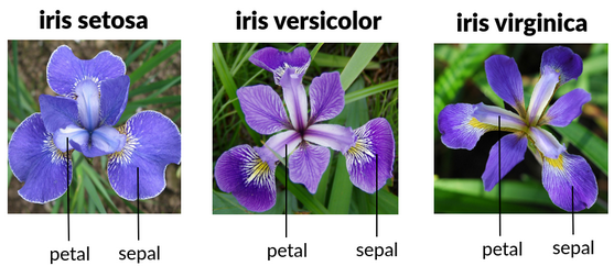
We will use the dataset iris.

data(iris)
head(iris)

  Sepal.Length Sepal.Width Petal.Length Petal.Width Species
1          5.1         3.5          1.4         0.2  setosa
2          4.9         3.0          1.4         0.2  setosa
3          4.7         3.2          1.3         0.2  setosa
4          4.6         3.1          1.5         0.2  setosa
5          5.0         3.6          1.4         0.2  setosa
6          5.4         3.9          1.7         0.4  setosa

dim(iris)

[1] 150   5

There are 5 variables and 150 individuals.

4 quantitative variables :

• Sepal.Length
• Sepal.Width
  
• Petal.Length
  
• Petal.Width

1 qualitative variable :

• Species

Univariate statistics

To have a global view : summary

summary(iris)

  Sepal.Length    Sepal.Width     Petal.Length    Petal.Width   
 Min.   :4.300   Min.   :2.000   Min.   :1.000   Min.   :0.100  
 1st Qu.:5.100   1st Qu.:2.800   1st Qu.:1.600   1st Qu.:0.300  
 Median :5.800   Median :3.000   Median :4.350   Median :1.300  
 Mean   :5.843   Mean   :3.057   Mean   :3.758   Mean   :1.199  
 3rd Qu.:6.400   3rd Qu.:3.300   3rd Qu.:5.100   3rd Qu.:1.800  
 Max.   :7.900   Max.   :4.400   Max.   :6.900   Max.   :2.500  
       Species  
 setosa    :50  
 versicolor:50  
 virginica :50  
                
                
                

The command summary gives us :

• for the quantitative variables :
  • the minimum
  • the 1st quartile
  • the median
  • the mean
  • the 3rd quartile
  • the maximum

• for the qualitative variables :
  • the number of observations in each category

Using describe for data summaries :

library(Hmisc)
describe(iris)

iris 

 5  Variables      150  Observations
--------------------------------------------------------------------------------
Sepal.Length 
       n  missing distinct     Info     Mean  pMedian      Gmd      .05 
     150        0       35    0.998    5.843      5.8   0.9462    4.600 
     .10      .25      .50      .75      .90      .95 
   4.800    5.100    5.800    6.400    6.900    7.255 

lowest : 4.3 4.4 4.5 4.6 4.7, highest: 7.3 7.4 7.6 7.7 7.9
--------------------------------------------------------------------------------
Sepal.Width 
       n  missing distinct     Info     Mean  pMedian      Gmd      .05 
     150        0       23    0.992    3.057     3.05   0.4872    2.345 
     .10      .25      .50      .75      .90      .95 
   2.500    2.800    3.000    3.300    3.610    3.800 

lowest : 2   2.2 2.3 2.4 2.5, highest: 3.9 4   4.1 4.2 4.4
--------------------------------------------------------------------------------
Petal.Length 
       n  missing distinct     Info     Mean  pMedian      Gmd      .05 
     150        0       43    0.998    3.758     3.65    1.979     1.30 
     .10      .25      .50      .75      .90      .95 
    1.40     1.60     4.35     5.10     5.80     6.10 

lowest : 1   1.1 1.2 1.3 1.4, highest: 6.3 6.4 6.6 6.7 6.9
--------------------------------------------------------------------------------
Petal.Width 
       n  missing distinct     Info     Mean  pMedian      Gmd      .05 
     150        0       22     0.99    1.199      1.2   0.8676      0.2 
     .10      .25      .50      .75      .90      .95 
     0.2      0.3      1.3      1.8      2.2      2.3 

lowest : 0.1 0.2 0.3 0.4 0.5, highest: 2.1 2.2 2.3 2.4 2.5
--------------------------------------------------------------------------------
Species 
       n  missing distinct 
     150        0        3 
                                           
Value          setosa versicolor  virginica
Frequency          50         50         50
Proportion      0.333      0.333      0.333
--------------------------------------------------------------------------------

• The Hmisc package provides the describe function to quickly summarize a dataset.

• For quantitative variables, it reports :
  • number of observations
  • missing values
  • mean
  • quantiles (5%, 10%, 25%, 50%, 75%, 90%, 95%)
  • 5 lowest and 5 highest values

• For qualitative variables, it reports :
  • number of observations
  • missing values
  • number of modalities
  • frequency and proportion of each modality

Quantitative variables

For each quantitative variable, it is also possible to obtain the following statistics separately.

• the sum of all the modalities in Sepal.Length

sum(iris$Sepal.Length)

[1] 876.5

• the mean of the variable Sepal.Length

mean(iris$Sepal.Length)

[1] 5.843333

• the variance of the variable Sepal.Length

var(iris$Sepal.Length)

[1] 0.6856935

• the standard deviation of the variable Sepal.Length

sd(iris$Sepal.Length)

[1] 0.8280661

• the minimum of the variable Sepal.Length

min(iris$Sepal.Length)

[1] 4.3

• the maximum of the variable Sepal.Length

max(iris$Sepal.Length)

[1] 7.9

• the median of the variable Sepal.Length

median(iris$Sepal.Length)

[1] 5.8

• the quantiles of the variable Sepal.Length

quantile(iris$Sepal.Length)

  0%  25%  50%  75% 100% 
 4.3  5.1  5.8  6.4  7.9 

• the number of modalities in the variable Sepal.Length

length(iris$Sepal.Length)

[1] 150

Chart representations

• A first representation is to use a boxplot
  
• Graphical way to summarize a quantitative variable
• Show its distribution, central tendency, and spread, including outliers.

Components of a Boxplot :

1. Median (Q2)
   • The line inside the box represents the median — the middle value of the data.
     
   • It divides the data into two equal sets.
2. Quartiles (Q1 and Q3)
   • Q1 (bottom of the box): 25% of the data is below this value.
     
   • Q3 (top of the box): 75% of the data is below this value.
     
   • The box shows the interquartile range (IQR = Q3 − Q1), which contains the middle 50% of the data.
3. Whiskers
   • Lines extending from the box to the minimum and maximum values within a certain range (usually 1.5 × IQR from Q1 and Q3)
4. Outliers
   • Points outside the whiskers plotted individually.
     
   • Represent values that are unusually high or low compared to the rest of the data.

boxplot(iris$Sepal.Length, col = c("yellow"),main = "Boxplot", ylab = "Sepal Length")

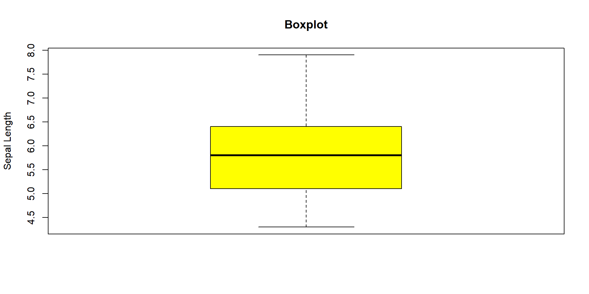
Also possible to represent many boxplot on the same plot

boxplot(iris[,c('Sepal.Length','Sepal.Width','Petal.Length','Petal.Width')],
        col = c("yellow"),                 #Pour la couleur
        main = paste("Boxplot"),     #Pour le titre
        ylab = "Length and width")              #Pour le titre de l’axe des ordonnées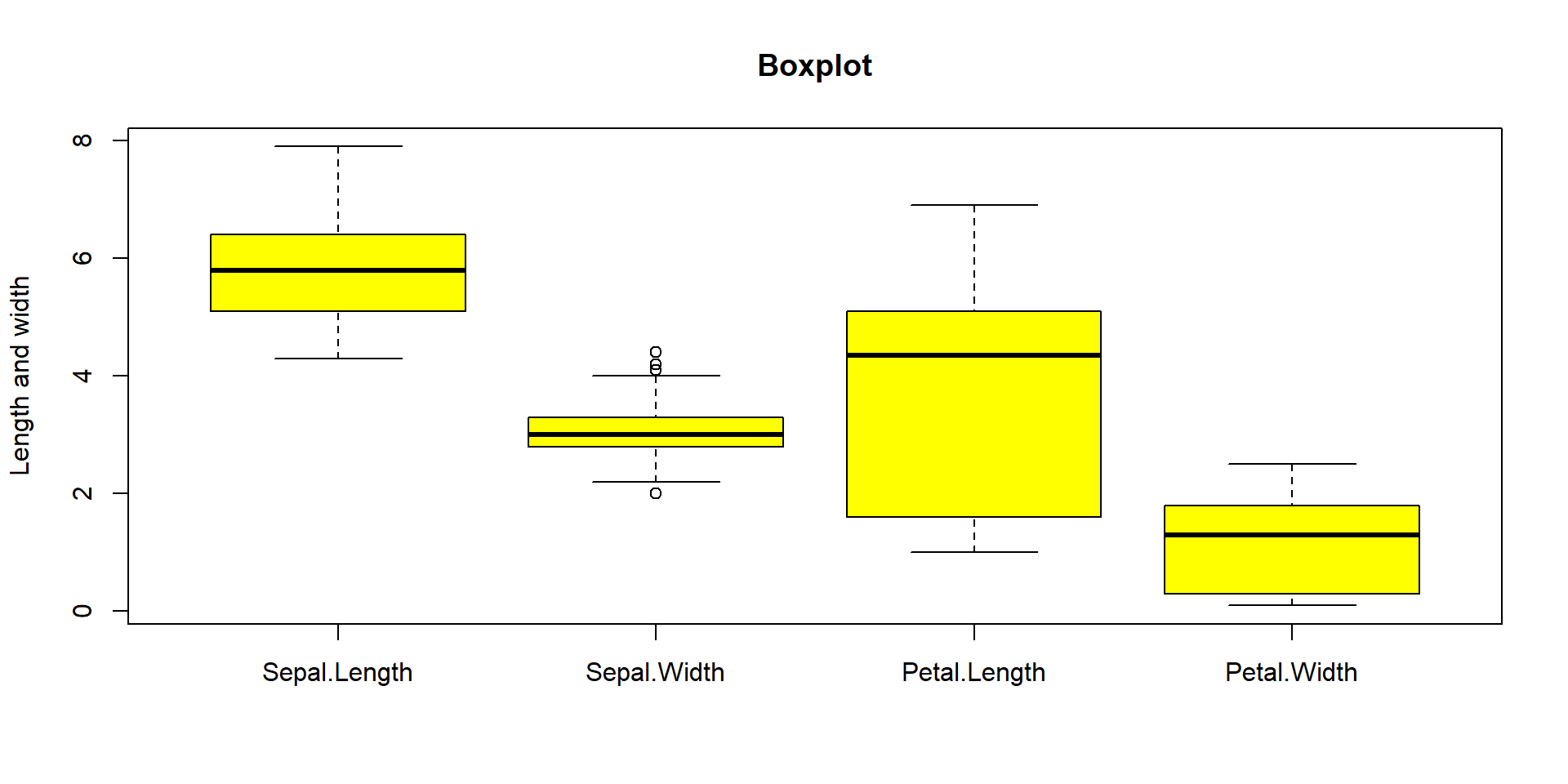

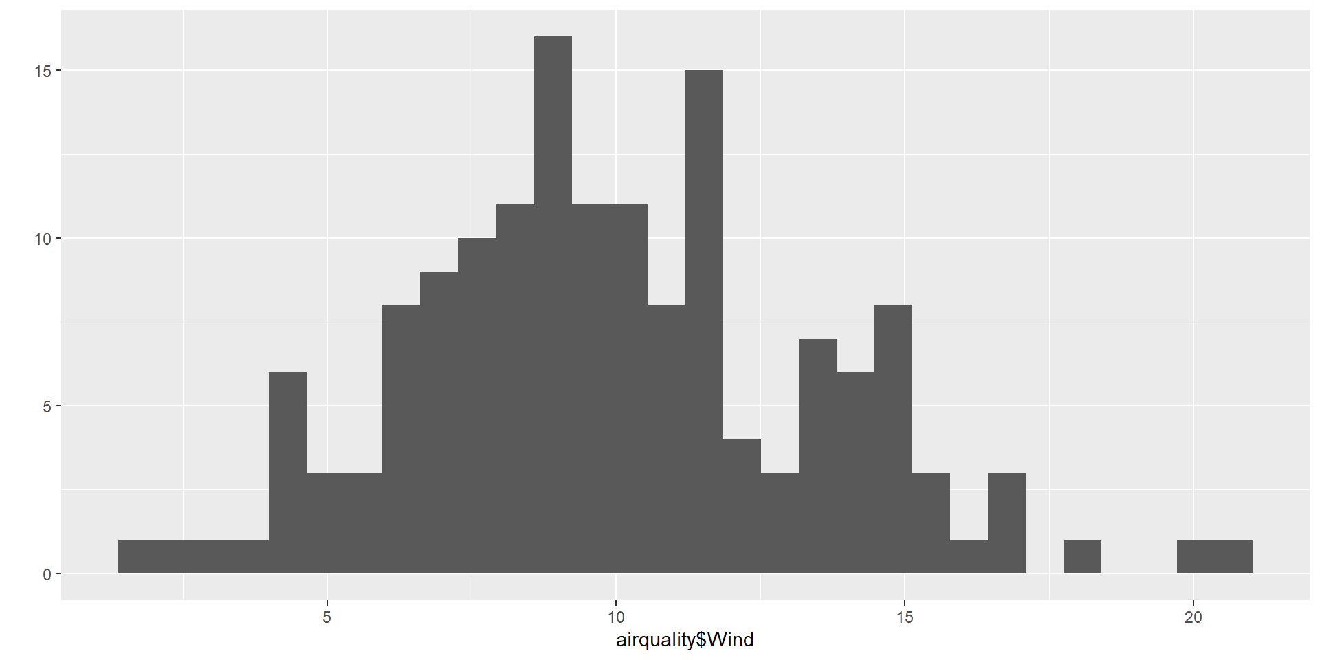
A usual graph is the histogram. It is a type of bar graph that represents the distribution of a quantitative variable.

Key Features

• Bins (Intervals):
  The x-axis is divided into continuous intervals called bins, each representing a range of values.

• Frequency:
  The y-axis shows the number of observations (frequency) in each bin.

• Bars:
  Each bin is represented by a bar.
  The height of the bar corresponds to the frequency.
  Bars touch each other because the data is continuous.

• Distribution Shape:
  A histogram helps visualize the shape of the data:

  • Symmetric or skewed
    
  • Uniform (flat)
    
  • Bimodal (two peaks)
    
  • Unimodal (one peak)

Why using an histogram ?

• Understand the shape of the data.
  
• Detect patterns, skewness, or clusters.
  
• Identify outliers or unusual gaps.

hist(iris$Sepal.Length, 
      col = c("orange"),
      main = paste("Histogramme pour la variable Sepal.Length"),
      ylab = "Effectifs",
      xlab = "Longueur du sépale")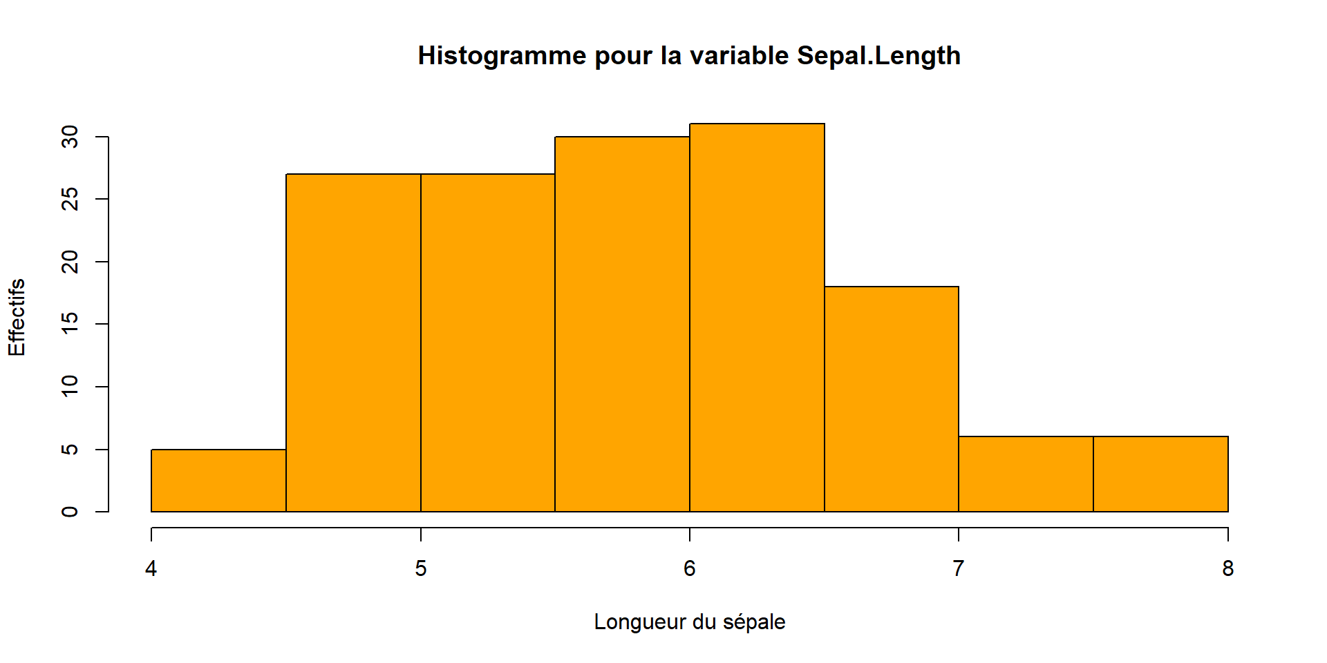

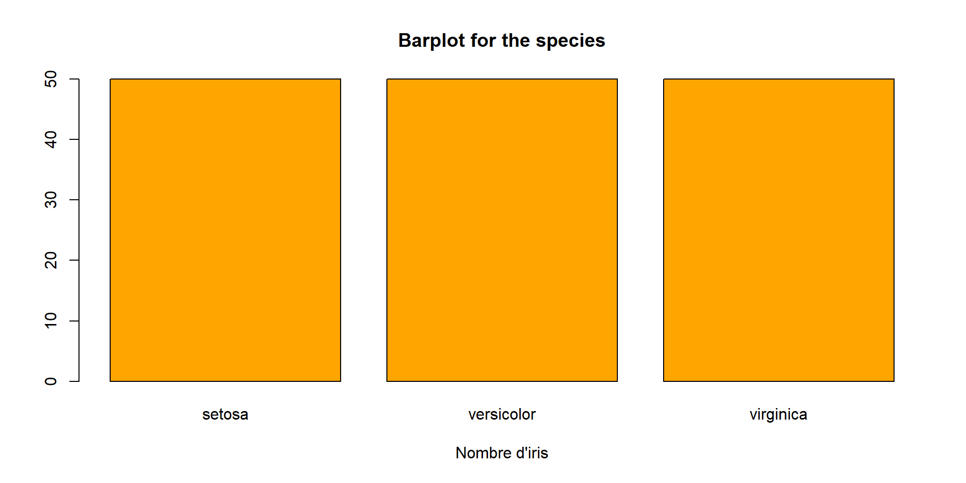
Qualitative variables

• the command table summarize categorical data by counting the frequency of each unique value
• It creates a contingency table, which is very useful in statistics for understanding distributions

table_Species<-table(iris$Species)
table_Species

    setosa versicolor  virginica 
        50         50         50 

The same with the proportions :

prop.table(table_Species)

    setosa versicolor  virginica 
 0.3333333  0.3333333  0.3333333 

and finally we can draw the bar plot for this variable

barplot(table_Species, main="Barplot for the species", 
        xlab="Nombre d'iris",
        col="orange")

Bivariate statistics

• Summarize and describe the relationship between two variables
  
• Explore how one variable changes with respect to another

Three types of situations :

1. Quantitative – Quantitative : Both variables are numeric
2. Quantitative – Qualitative : One numeric, one categorical
3. Qualitative – Qualitative : Both categorical

Quantitative VS Quantitative

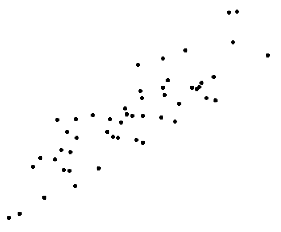
A scatter plot is one of the most commonly used tools to visualize the relationship between two quantitative variables.

plot(iris$Sepal.Length,iris$Sepal.Width)

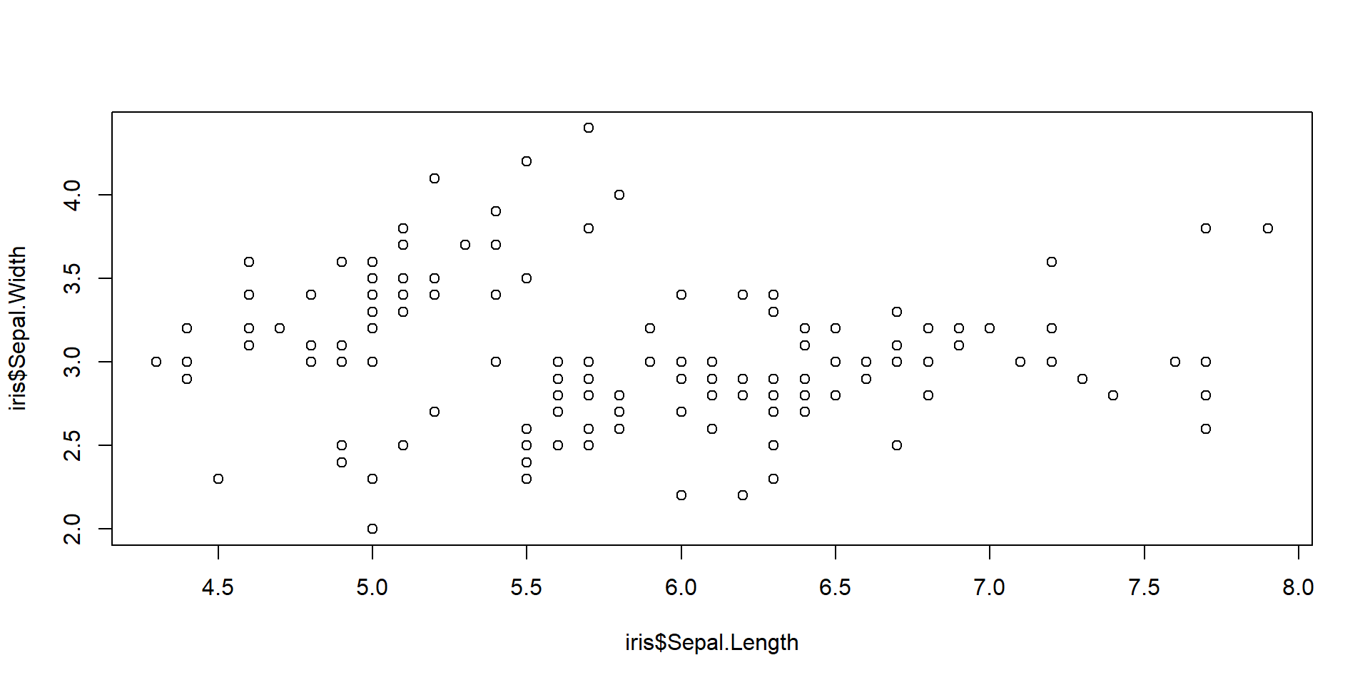
It can give an idea of the relationship between the 2 variables.

Quantitative VS Qualitative

The command by gives statistics summary for each modality of the qualitative variable

by(iris[,1:4], INDICES=iris[,"Species"], FUN=summary)

iris[, "Species"]: setosa
  Sepal.Length    Sepal.Width     Petal.Length    Petal.Width   
 Min.   :4.300   Min.   :2.300   Min.   :1.000   Min.   :0.100  
 1st Qu.:4.800   1st Qu.:3.200   1st Qu.:1.400   1st Qu.:0.200  
 Median :5.000   Median :3.400   Median :1.500   Median :0.200  
 Mean   :5.006   Mean   :3.428   Mean   :1.462   Mean   :0.246  
 3rd Qu.:5.200   3rd Qu.:3.675   3rd Qu.:1.575   3rd Qu.:0.300  
 Max.   :5.800   Max.   :4.400   Max.   :1.900   Max.   :0.600  
------------------------------------------------------------ 
iris[, "Species"]: versicolor
  Sepal.Length    Sepal.Width     Petal.Length   Petal.Width   
 Min.   :4.900   Min.   :2.000   Min.   :3.00   Min.   :1.000  
 1st Qu.:5.600   1st Qu.:2.525   1st Qu.:4.00   1st Qu.:1.200  
 Median :5.900   Median :2.800   Median :4.35   Median :1.300  
 Mean   :5.936   Mean   :2.770   Mean   :4.26   Mean   :1.326  
 3rd Qu.:6.300   3rd Qu.:3.000   3rd Qu.:4.60   3rd Qu.:1.500  
 Max.   :7.000   Max.   :3.400   Max.   :5.10   Max.   :1.800  
------------------------------------------------------------ 
iris[, "Species"]: virginica
  Sepal.Length    Sepal.Width     Petal.Length    Petal.Width   
 Min.   :4.900   Min.   :2.200   Min.   :4.500   Min.   :1.400  
 1st Qu.:6.225   1st Qu.:2.800   1st Qu.:5.100   1st Qu.:1.800  
 Median :6.500   Median :3.000   Median :5.550   Median :2.000  
 Mean   :6.588   Mean   :2.974   Mean   :5.552   Mean   :2.026  
 3rd Qu.:6.900   3rd Qu.:3.175   3rd Qu.:5.875   3rd Qu.:2.300  
 Max.   :7.900   Max.   :3.800   Max.   :6.900   Max.   :2.500  

The psych package, using describe, allows to compute the following statistics :

• Number of observations

• Mean

• Standard deviation
  

• Median

• Trimmed mean (calculated by removing the 5 smallest and 5 largest values)

• Median absolute deviation (robust measure of spread, defined as the median of the absolute differences between each value and the dataset’s median)

• Minimum
  

• Maximum
  

• Range (maximum − minimum)

• Skewness (measures the asymmetry of a distribution, indicating whether the data are skewed to the left (negative) or right (positive) )

• Kurtosis (measures the “tailedness” of a distribution, indicating whether data have heavy tails (outliers) or light tails compared to a normal distribution)

• Standard error (measures how much a sample mean is likely to vary from the true population mean)

library(psych)
describeBy(iris, group=iris$Species)

 Descriptive statistics by group 
group: setosa
             vars  n mean   sd median trimmed  mad min max range skew kurtosis
Sepal.Length    1 50 5.01 0.35    5.0    5.00 0.30 4.3 5.8   1.5 0.11    -0.45
Sepal.Width     2 50 3.43 0.38    3.4    3.42 0.37 2.3 4.4   2.1 0.04     0.60
Petal.Length    3 50 1.46 0.17    1.5    1.46 0.15 1.0 1.9   0.9 0.10     0.65
Petal.Width     4 50 0.25 0.11    0.2    0.24 0.00 0.1 0.6   0.5 1.18     1.26
Species         5 50 1.00 0.00    1.0    1.00 0.00 1.0 1.0   0.0  NaN      NaN
               se
Sepal.Length 0.05
Sepal.Width  0.05
Petal.Length 0.02
Petal.Width  0.01
Species      0.00
------------------------------------------------------------ 
group: versicolor
             vars  n mean   sd median trimmed  mad min max range  skew kurtosis
Sepal.Length    1 50 5.94 0.52   5.90    5.94 0.52 4.9 7.0   2.1  0.10    -0.69
Sepal.Width     2 50 2.77 0.31   2.80    2.78 0.30 2.0 3.4   1.4 -0.34    -0.55
Petal.Length    3 50 4.26 0.47   4.35    4.29 0.52 3.0 5.1   2.1 -0.57    -0.19
Petal.Width     4 50 1.33 0.20   1.30    1.32 0.22 1.0 1.8   0.8 -0.03    -0.59
Species         5 50 2.00 0.00   2.00    2.00 0.00 2.0 2.0   0.0   NaN      NaN
               se
Sepal.Length 0.07
Sepal.Width  0.04
Petal.Length 0.07
Petal.Width  0.03
Species      0.00
------------------------------------------------------------ 
group: virginica
             vars  n mean   sd median trimmed  mad min max range  skew kurtosis
Sepal.Length    1 50 6.59 0.64   6.50    6.57 0.59 4.9 7.9   3.0  0.11    -0.20
Sepal.Width     2 50 2.97 0.32   3.00    2.96 0.30 2.2 3.8   1.6  0.34     0.38
Petal.Length    3 50 5.55 0.55   5.55    5.51 0.67 4.5 6.9   2.4  0.52    -0.37
Petal.Width     4 50 2.03 0.27   2.00    2.03 0.30 1.4 2.5   1.1 -0.12    -0.75
Species         5 50 3.00 0.00   3.00    3.00 0.00 3.0 3.0   0.0   NaN      NaN
               se
Sepal.Length 0.09
Sepal.Width  0.05
Petal.Length 0.08
Petal.Width  0.04
Species      0.00

For each quantitative variable, possible to plot the boxplot for all the modalities of the qualitative variable.

boxplot(iris$Sepal.Length ~ iris$Species,
        col = c("yellow"),
        main = paste("Boxplot pour la variable Sepal.Length, par espèce d'iris"),
        ylab = "Quantiles")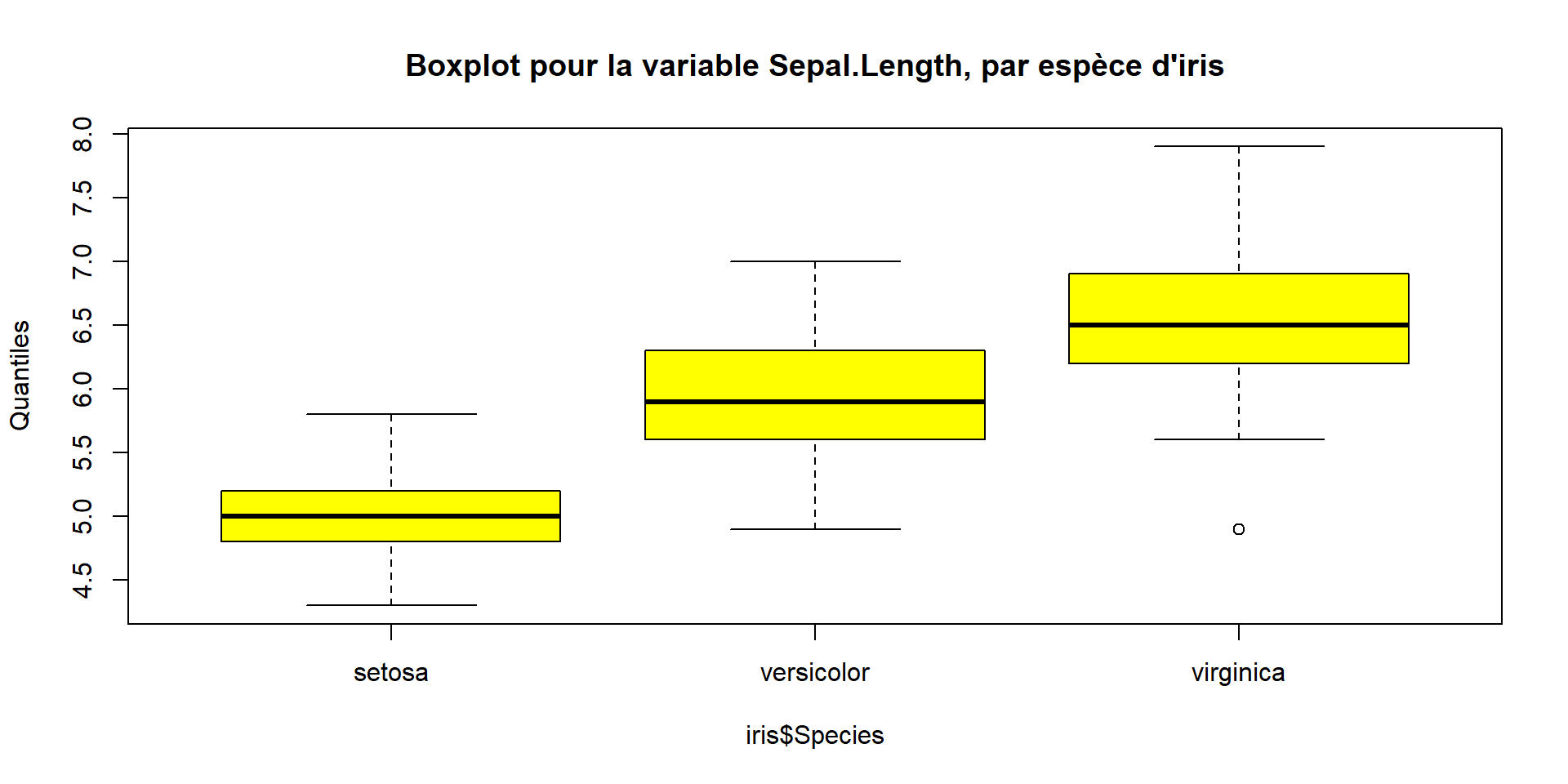

Qualitative VS Qualitative

First we create another qualitative variable for our example : Sepal.Length_cat

iris$Sepal.Length_cat[iris$Sepal.Length<=5]<-"petit"
iris$Sepal.Length_cat[iris$Sepal.Length<=6 & iris$Sepal.Length>5]<-"moyen"
iris$Sepal.Length_cat[iris$Sepal.Length>6]<-"grand"

Now we have

head(iris)

  Sepal.Length Sepal.Width Petal.Length Petal.Width Species Sepal.Length_cat
1          5.1         3.5          1.4         0.2  setosa            moyen
2          4.9         3.0          1.4         0.2  setosa            petit
3          4.7         3.2          1.3         0.2  setosa            petit
4          4.6         3.1          1.5         0.2  setosa            petit
5          5.0         3.6          1.4         0.2  setosa            petit
6          5.4         3.9          1.7         0.4  setosa            moyen

We get contingency table with table

table_Species_Length<-table(iris$Species,iris$Sepal.Length_cat)
table_Species_Length

            
             grand moyen petit
  setosa         0    22    28
  versicolor    20    27     3
  virginica     41     8     1

the sum for each modality of Species

margin.table(table_Species_Length, 1) 

    setosa versicolor  virginica 
        50         50         50 

the sum for each modality of Sepal.Length_cat

margin.table(table_Species_Length, 2) 

grand moyen petit 
   61    57    32 

the same with proportions (with respect to the total number of observations)

prop.table(table_Species_Length)

            
                   grand       moyen       petit
  setosa     0.000000000 0.146666667 0.186666667
  versicolor 0.133333333 0.180000000 0.020000000
  virginica  0.273333333 0.053333333 0.006666667

now with respect to the number of observations for each row

prop.table(table_Species_Length, 1) # proportion sur l'effectif total de la ligne

            
             grand moyen petit
  setosa      0.00  0.44  0.56
  versicolor  0.40  0.54  0.06
  virginica   0.82  0.16  0.02

and finally with respect to the number of each column

prop.table(table_Species_Length, 2) # proportion sur l'effectif total de la colonne

            
                 grand     moyen     petit
  setosa     0.0000000 0.3859649 0.8750000
  versicolor 0.3278689 0.4736842 0.0937500
  virginica  0.6721311 0.1403509 0.0312500

The gmodels package allows to create more advanced tables.

library(gmodels)
CrossTable(iris$Species,iris$Sepal.Length_cat,prop.chisq=FALSE,chisq=FALSE,expected=FALSE)

 
   Cell Contents
|-------------------------|
|                       N |
|           N / Row Total |
|           N / Col Total |
|         N / Table Total |
|-------------------------|

 
Total Observations in Table:  150 

 
             | iris$Sepal.Length_cat 
iris$Species |     grand |     moyen |     petit | Row Total | 
-------------|-----------|-----------|-----------|-----------|
      setosa |         0 |        22 |        28 |        50 | 
             |     0.000 |     0.440 |     0.560 |     0.333 | 
             |     0.000 |     0.386 |     0.875 |           | 
             |     0.000 |     0.147 |     0.187 |           | 
-------------|-----------|-----------|-----------|-----------|
  versicolor |        20 |        27 |         3 |        50 | 
             |     0.400 |     0.540 |     0.060 |     0.333 | 
             |     0.328 |     0.474 |     0.094 |           | 
             |     0.133 |     0.180 |     0.020 |           | 
-------------|-----------|-----------|-----------|-----------|
   virginica |        41 |         8 |         1 |        50 | 
             |     0.820 |     0.160 |     0.020 |     0.333 | 
             |     0.672 |     0.140 |     0.031 |           | 
             |     0.273 |     0.053 |     0.007 |           | 
-------------|-----------|-----------|-----------|-----------|
Column Total |        61 |        57 |        32 |       150 | 
             |     0.407 |     0.380 |     0.213 |           | 
-------------|-----------|-----------|-----------|-----------|

 

Probability and sampling

coming !

Probability

coming !

Sampling

coming !

Statistical tests

• Tools to decide if data supports an hypothesis
  
• Compare observed results with what is expected under an hypothesis
• Help control errors
• Guide data-driven decisions

Statistical hypothesis tests

A procedure to know if something has changed in a poputalion.

• Collect a sample that is representative of the whole population.
  
• State the hypothesis you want to test.

A very good video about statistical hypothesis testing.

The Hypothesis

Two Competing Hypotheses :

1. Null hypothesis H0 :
   The conservative hypothesis ; “There is nothing going on !”

2. Alternative hypothesis H1 :
   “There is something going on”

Type 1 and Type 2 Errors

In a hypothesis test, we make a decision about which of H0 or H1 might be true, but our decision might be incorrect !

	We fail to reject \(H_0\)	We reject \(H_0\)
In reality \(H_0\) is true	\(\checkmark\)	Type 1 Error \(\alpha\)
In reality \(H_1\) is true	Type 2 Error \(\beta\)	\(\checkmark\)

• Goal : Minimizing Type I error (\(\alpha\)) and Type II error \((\beta)\)
  
• Many ways to minimize a problem with 2 parameters.

Type I error > Type II error

Type I error (\(\alpha\)) and Type II error \((\beta)\) DO NOT HAVE THE SAME IMPACT on the situation being tested !!
Type I error (\(\alpha\)) is way more harmful !

Therefore we fix \(\alpha\) as small as we like, and try to minimize \(\beta\).

“Inside” a statistical hypothesis test

Important

The next step of hypothesis testing is to weigh the evidence !

Could these data plausibly have happened by chance if the H0 was true ?

The procedure :

• We collect data in our population

• We import our data in RStudio

• We use the right test

• We “write” the test we chose

• And according to the p-value we get, we can accept or reject H0

  • If p-value > \(\alpha\), then we accept H0
  • If p-value < \(\alpha\), then we reject H0

What remains to be learned?

We now need to learn which test to choose, how to choose it, and how to implement it on RStudio.
cf. next slides

Example

A first example of hypothesis testing within R.

In this video, the author tackle two questions relating to R’s built-in airquality data set. We’ll view this set as a simple random sample of air quality measurements in New York City.

Questions

• An official claims that the average wind speed in the city is 9 miles per hour. Is this plausible ?
  
• A certain solar array will only be cost-effective if mean solar radiation is over 175 Langleys. Would it be a sound investment in light of this data?

Let’s go work on RStudio.

library(tidyverse)
head(airquality)

  Ozone Solar.R Wind Temp Month Day
1    41     190  7.4   67     5   1
2    36     118  8.0   72     5   2
3    12     149 12.6   74     5   3
4    18     313 11.5   62     5   4
5    NA      NA 14.3   56     5   5
6    28      NA 14.9   66     5   6

dim(airquality)

[1] 153   6

The dataset used here is called airquality. There are 6 variables and 153 individuals.

• Ozone
  
• Solar.R
  
• Wind

• Temp
• Month
  
• Day

Question 1

In order to answer the first question, we look at Wind

qplot(airquality$Wind, geom = "histogram")

H0 : the null hypotesis

Here the null hypotesis is that the average wind speed in the city is 9 miles per hour.

We will use here a t.test. We explain more about this test in next slides.

t.test(airquality$Wind, mu = 9)

    One Sample t-test

data:  airquality$Wind
t = 3.3619, df = 152, p-value = 0.0009794
alternative hypothesis: true mean is not equal to 9
95 percent confidence interval:
  9.394804 10.520229
sample estimates:
mean of x 
 9.957516 

We get a p-value \(\simeq \ 0.0010 \ \simeq \ 0.1 \% \ < \alpha = 5 \%\)

Conclusion

We can therefore reject H0.

The average wind speed in the city is NOT 9 miles per hour.

Question 2

In order to answer the second question, we look at Solar.R

qplot(airquality$Solar.R, geom = "histogram")

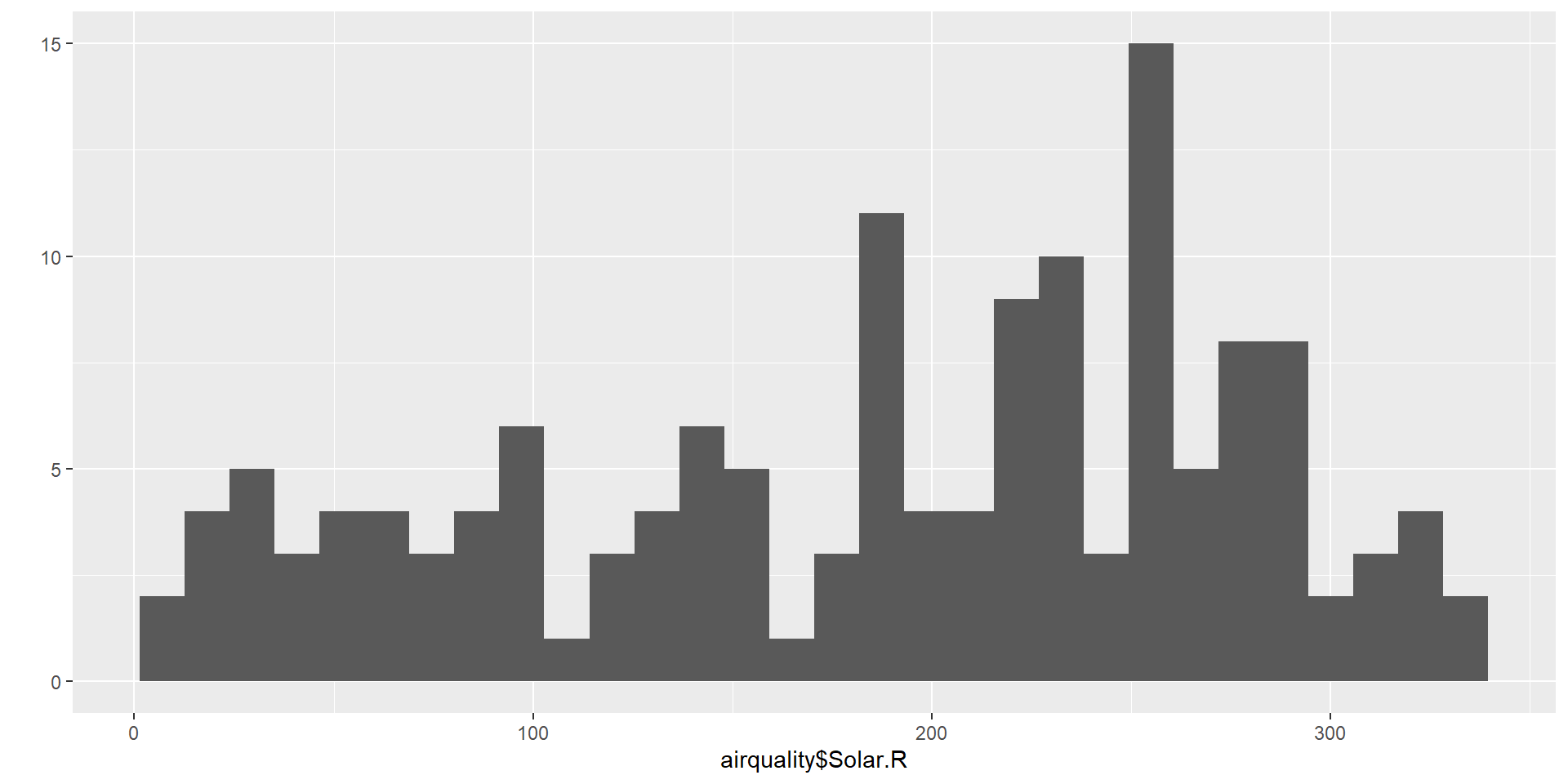
H0 : the null hypotesis

Here the null hypotesis is that the mean solar radiation is 175 Langleys.
And the alternative hypothesis H1 is that this mean is greater than 175 Langleys.

Again we will use here a t.test.

t.test(airquality$Solar.R, mu = 175, alternative = "greater")

    One Sample t-test

data:  airquality$Solar.R
t = 1.4667, df = 145, p-value = 0.07232
alternative hypothesis: true mean is greater than 175
95 percent confidence interval:
 173.5931      Inf
sample estimates:
mean of x 
 185.9315 

We get a p-value \(\simeq \ 0.072 \ \simeq \ 7.2 \% \ > \alpha = 5 \%\)

Conclusion

We can therefore accept H0.

Parametric and nonparametric statistical tests

• Parametric tests : requirements about the shape of the populations involved

• Non-parametric tests do not require that samples come from populations with normal distributions or have any other particular distributions.

Non-parametric tests are called distribution-free tests.

An interesting on the difference between parametric and non-parametric test.

Parametric tests < Non-parametric tests

• Nonparametric methods can be applied to a wide variety of situations because they do not have the more rigid requirements of the corresponding parametric methods.

• Unlike parametric methods, nonparametric methods can often be applied to categorical data.

• Nonparametric methods usually involve simpler computations than the corresponding parametric methods.

Parametric tests > Non-parametric tests

• Nonparametric methods tend to waste information

• Nonparametric tests are not as efficient as parametric tests

• With a nonparametric test we need stronger evidence (such as a larger sample or greater differences) before we reject a null hypothesis.

Chi-squared tests

• There are three types of Chi-squared tests.

• We write Chi-squared OR \(\chi^2\).

\(\chi^2\) goodness-of-fit test

Non-parametric test

Dependent variable	/
Independant variable	Qualitative

Asumption :

• Observations must be independent

H0 : Null hypothesis

The population follows the specified distribution.

Example :

The author tackle two goodness-of-fit problems using R.

• One with different proportions
  
• One with same proportions

1st problem

• A college reports that
  • \(50 \%\) of the students in its statistics classes are freshmen,
  • \(30 \%\) are sophomores,
  • \(10 \%\) are juniors,
  • and \(10 \%\) are seniors.

A simple random sample of \(65\) such students has the following breakdown :

Freshman	Sophomore	Junior	Senior
28	24	9	4

Question

Does this constitute sufficient evidence to doubt the percentages reported by the college ?

We define the variable years sample

years = c(28, 24, 9, 4)

then the proportions expected from what the college did report

props = c(0.5, 0.3, 0.1, 0.1)

• Now we can perform our goodness-of-fit test.

• Here the null hypothesis is that the population follows the specified distribution, meaning the sample does agree with what the college did report.

chisq.test(years, p = props)

    Chi-squared test for given probabilities

data:  years
X-squared = 3.5846, df = 3, p-value = 0.31

• We get a p-value \(\simeq \ 0.31 \ \simeq \ 31 \% \ > \alpha\)

• Therefore we can accept H0.

• The sample made do not constitute sufficient evidence to doubt the percentages reported by the college
  

2nd problem

• 200 rolls of a die result in the following distribution:

1	2	3	4	5	6
28	30	22	31	38	51

Question

Should we conclude that the die is unfair ?

We define the variable years for the sample.

counts = c(28, 30, 22, 31, 38, 51)

• Given the theoretical proportion will be all the same, we do not need to define a vector for the proportions.

• Here H0 is that the die is fair.

chisq.test(counts)

    Chi-squared test for given probabilities

data:  counts
X-squared = 15.22, df = 5, p-value = 0.009463

• We get a p-value \(\simeq \ 0.001 \ \simeq \ 0.01 \% \ < \alpha\)

• Therefore we can reject H0.

• According to this test we are going to say that the die is unfair.

\(\chi^2\) test for homogeneity

Non-parametric test

Dependent variable	Qualitative
Independant variable	Qualitative

Asumption :

• Each population is at least 10 times as large as its respective sample
• The expected frequency count for each value is at least 5

H0 : Null hypothesis

The distribution of the categorical variable is the same for each subgroup or population

Example :

The author tackle one \(\chi^2\) test for homogeneity using R.

Problem

A random sample of students at two universities resulted in the following distribution of fields of study:

University	Business	Engineering	Liberal arts	Nursing
A	64	47	145	31
B	41	35	174	52

Question

Is it safe to conclude that the populations of students in the two schools have different distributions of fields of study?

• We define the vector students.

• From students we define the matrix m

students = c(64, 47, 145, 31, 41, 35, 174, 52)
m = matrix(students, nrow = 2, byrow = TRUE)
m

     [,1] [,2] [,3] [,4]
[1,]   64   47  145   31
[2,]   41   35  174   52

It’s optionnal, but can name the columns and rows.

colnames(m) = c("Business", "Engineering", "Liberal arts", "Nursing")
rownames(m) = c("A", "B")
m

  Business Engineering Liberal arts Nursing
A       64          47          145      31
B       41          35          174      52

• Now we can perform our \(\chi^2\) test for homogenity.

• Here the null hypothesis H0 is that the populations of students in the two schools have the same distribution of fields of study.

chisq.test(m)

    Pearson's Chi-squared test

data:  m
X-squared = 14.371, df = 3, p-value = 0.002441

• We get a p-value \(\simeq \ 0.002 \ \simeq \ 0.2 \% \ < \alpha\)

• Therefore we can reject H0.

• The populations of students in the two schools have different distributions of fields of study.

\(\chi^2\) test for independence

Non-parametric test

Dependent variable	Qualitative
Independant variable	Qualitative

Asumptions :

• Observations must be independent
• Relatively large sample size

H0 : Null hypothesis

There is no association between the two variables.

Example :

The author tackle a \(\chi^2\) test for independence using R.

The two variables are :

• the type of volunteer

• the amount of hours spend voluntering

Problem

In a volunteer group, adults 21 and older volunteer from one to nine hours each week to spend time with a disabled senior citizen. The program recruits among :
- community college students,

• four-year college students,

• and nonstudents.

In the table we have a sample of the adult volunteers and the number of hours they volunteer per week.

Type of Volunteer	1-3 Hours	4-6 Hours	7-9 Hours	Row Total
Community College Students	111	96	48	255
Four-Year College Students	96	133	61	290
Nonstudents	91	150	53	294
Column Total	298	379	162	839

Question

Is the number of hours volunteered independent of the type of volunteer?

We define the variable volunteers.

volunteers = matrix(c(111, 96, 48, 96, 133, 61, 91, 150, 53), byrow = TRUE, nrow = 3)
volunteers

     [,1] [,2] [,3]
[1,]  111   96   48
[2,]   96  133   61
[3,]   91  150   53

We name the columns and the rows.

rownames(volunteers) = c("Community College", "Four Year", "Nonstudent")
colnames(volunteers) = c("1-3 hours", "4-6 hours", "7-9 hours")
volunteers

                  1-3 hours 4-6 hours 7-9 hours
Community College       111        96        48
Four Year                96       133        61
Nonstudent               91       150        53

• Now we can perform our \(\chi^2\) indendence test.

• Here the null hypothesis is that the two variables are independent.

model = chisq.test(volunteers)
model

    Pearson's Chi-squared test

data:  volunteers
X-squared = 12.991, df = 4, p-value = 0.01132

• We get a p-value \(\simeq \ 0.01 \ \simeq \ 1 \% \ < \alpha\)

• Therefore we can reject H0.

• It does look like, according to this sample, that the number of hours volunteered is dependent of the type of volunteer.

Binomial test

Non-parametric test

Dependent variable	-
Independant variable	Qualitative (Binary)

Asumptions :

• Random samples
• Independent observations
• The variable of interest is binary (only two possible outcomes)
• The number of trials is fixed

H0 : Null hypothesis

The population proportion of one outcome equals some claimed value.

Example :

• The author tackle a binomial test to see if the proportion of leopards with a solid black coat color equals \(0.35\).

• We are going to do it using R.

Problem

According to a genetic model, \(35 \%\) of a certain subspecies of leopards have a solid black coat color.

• We believe this rate is lower for leopards living in a wildlife refuge.

• So we randomly select 9 unrelated leopards and find that only 1 has a solid black coat.

Question

Is there enough evidence to suggest that the rate is lower than \(35\%\) for leopards living in the refuge.

We define the variables

• leopards_sample

• leopards_black_coat

• model_proportion

leopards_sample = 9
leopards_black_coat = 1
model_proportion = 0.35

• Now we can perform our binomial test

• Here the null hypothesis H0 is that the rate is equal to \(45 \%\)

binom.test(leopards_black_coat, leopards_sample, p = model_proportion)

    Exact binomial test

data:  leopards_black_coat and leopards_sample
number of successes = 1, number of trials = 9, p-value = 0.1747
alternative hypothesis: true probability of success is not equal to 0.35
95 percent confidence interval:
 0.002809137 0.482496515
sample estimates:
probability of success 
             0.1111111 

• We get a p-value \(\simeq \ 0.17 \ \simeq \ 17 \% \ > \alpha\)

• Therefore we can accept H0.

• The rate of \(35 \%\) given by the genetic model seems to be correct

Tests for normality

To check for normality, :

• Graphical methods
  • Histogram
  • Boxplot
  • Density plot
  • QQ plot

• Statistical tests
  • Shapiro-Wilk test
  • Kolmogorov-Smirnov test

Graphical method

First we load the required packages

library(ggpubr)
library(ggplot2)
library(tidyverse)
library(palmerpenguins) # the dataset we are going to use

Histogram, density plot

It gives an idea on the chance for the variable to be normal.

We can plot at the same time :

• the histogram
• the density plot
• the theoretical normal distribution density

penguins.mean = mean(penguins$body_mass_g, na.rm = TRUE)
penguins.sd = sd(penguins$body_mass_g, na.rm = TRUE)

ggplot(penguins, aes(x = body_mass_g)) +
  # Colors for the two curves
  scale_color_manual(name = "Legend",
                     values = c("Density plot" = "#3AC275",
                                "Theoretical normal distribution" = "#FF59A9")) +
  # Theretical curve
  geom_line(stat = "function",
            fun = dnorm, #normal distribution density function
            args = list(mean = penguins.mean, sd = penguins.sd),
            aes(color = "Theoretical normal distribution"),
            linewidth = 1.8) +
  # Histogram
  geom_histogram(aes(y = after_stat(density)), #plot histogram using density, not counts
                na.rm = TRUE,
                bins = 40,
                alpha=0.7, 
                fill="#33AADE", 
                color="#332F61") +
  # Density plot
  geom_density(na.rm = TRUE,
               alpha=0.4,
               aes(color = "Density plot"),
               linewidth = 1,
               fill="#7EA38F") +
  # Title-s
  labs(title = "Histogram", x = "Body mass (g)", y = "Density") +
  # Side legend
  theme(legend.position = "right")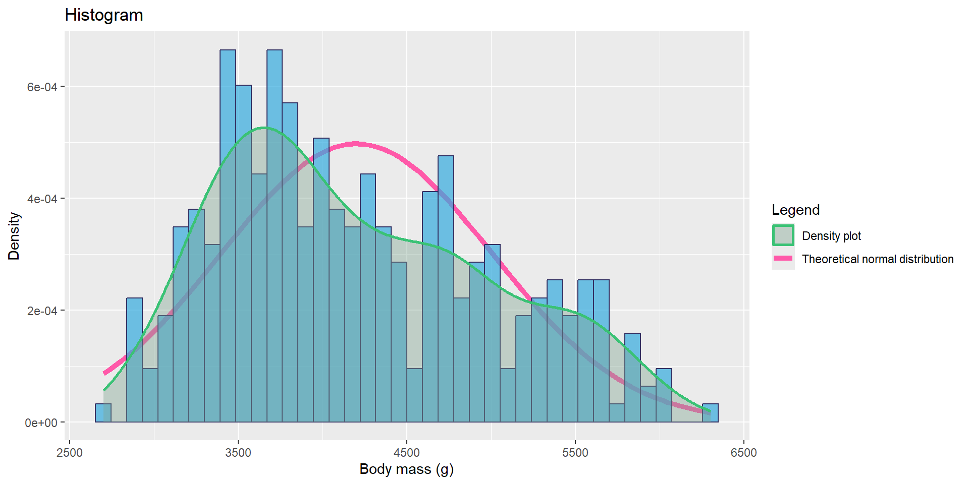

The variable body_mass_g does not look like it follows a normal distribution.

Boxplot (and violin plot)

• Boxplot : A normal distribution is symmetric, thus if :
  • the median line inside the box is roughly in the center of the box,
  • and the length of the whiskers are roughly equal on both sides, then we might have a normal distribution
• Violin plot :
  • The width at a given value represents the density (how many points are near that value).
  • Wide sections \(\to\) many observations.
  • Narrow sections \(\to\) few observations

library(ggpubr)
library(dplyr)
library(palmerpenguins)

# Remove rows with NA in body_mass_g
penguins_clean <- penguins %>%
  filter(!is.na(body_mass_g))

# Create the plot
ggviolin(penguins_clean, 
         y = "body_mass_g",
         fill = "#00AFBB",
         add = "boxplot",
         add.params = list(fill = "white")) +
  labs(title = "hhhhhh",
       y = "qjmfsjd",
       x = "lhqkfjs") +
  theme_minimal() +
  stat_summary(fun = mean, geom = "point", shape = 23, size = 3, fill = "red")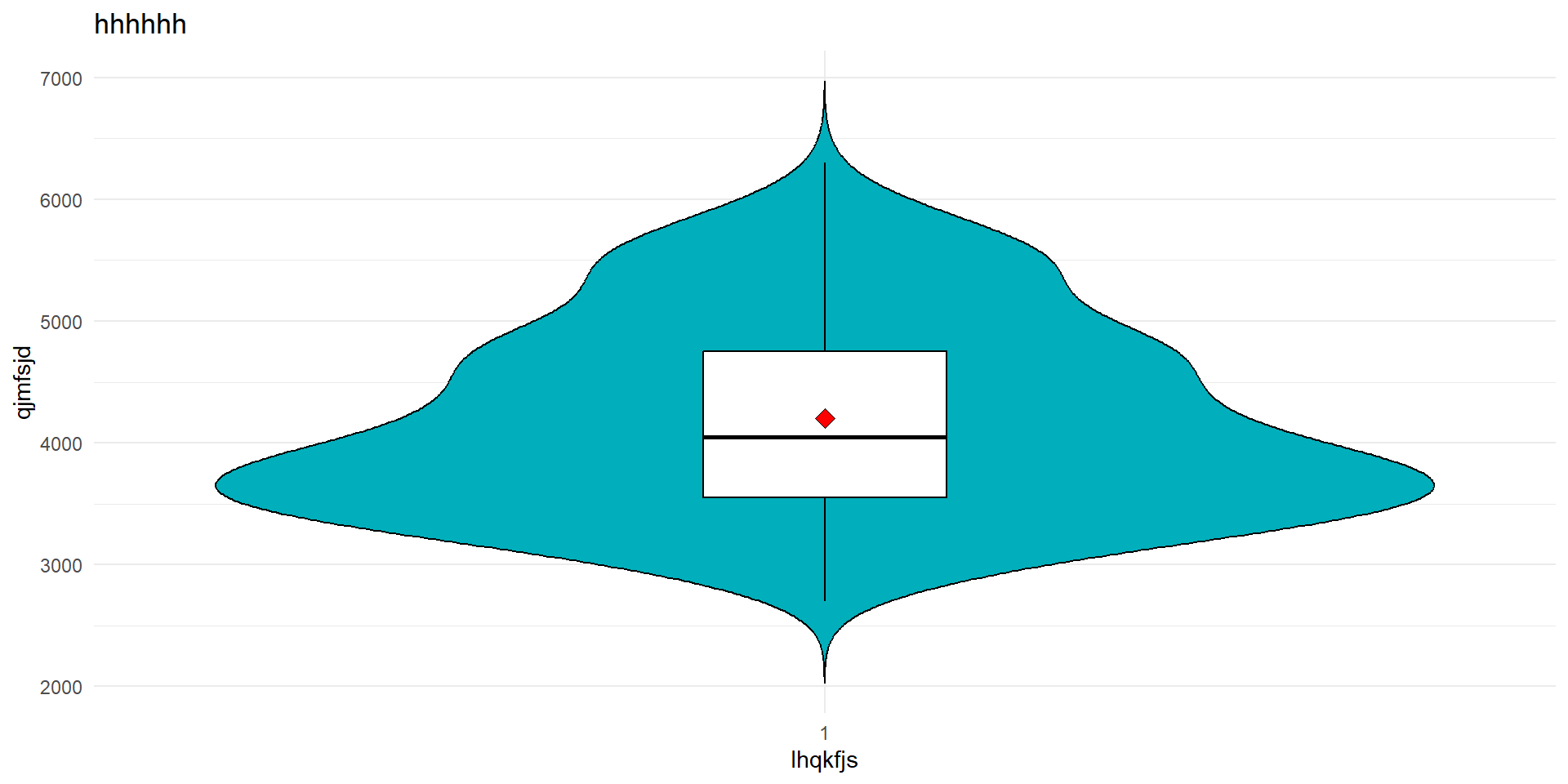

Same conclusion the variable body_mass_g does not look like it follows a normal distribution.

QQ plot

• A Q–Q plot compares the quantiles of your data to the quantiles of a theoretical normal distribution.
• If the data are normally distributed, the points should fall roughly on a straight diagonal line.

# Remove NA values from body_mass_g
body_mass <- na.omit(penguins$body_mass_g)

# Create a QQ plot
ggqqplot(body_mass,
         title = "QQ Plot of Penguin Body Mass",
         xlab = "Theoretical Quantiles",
         ylab = "Sample Quantiles",
         color = "blue",
         shape = 19)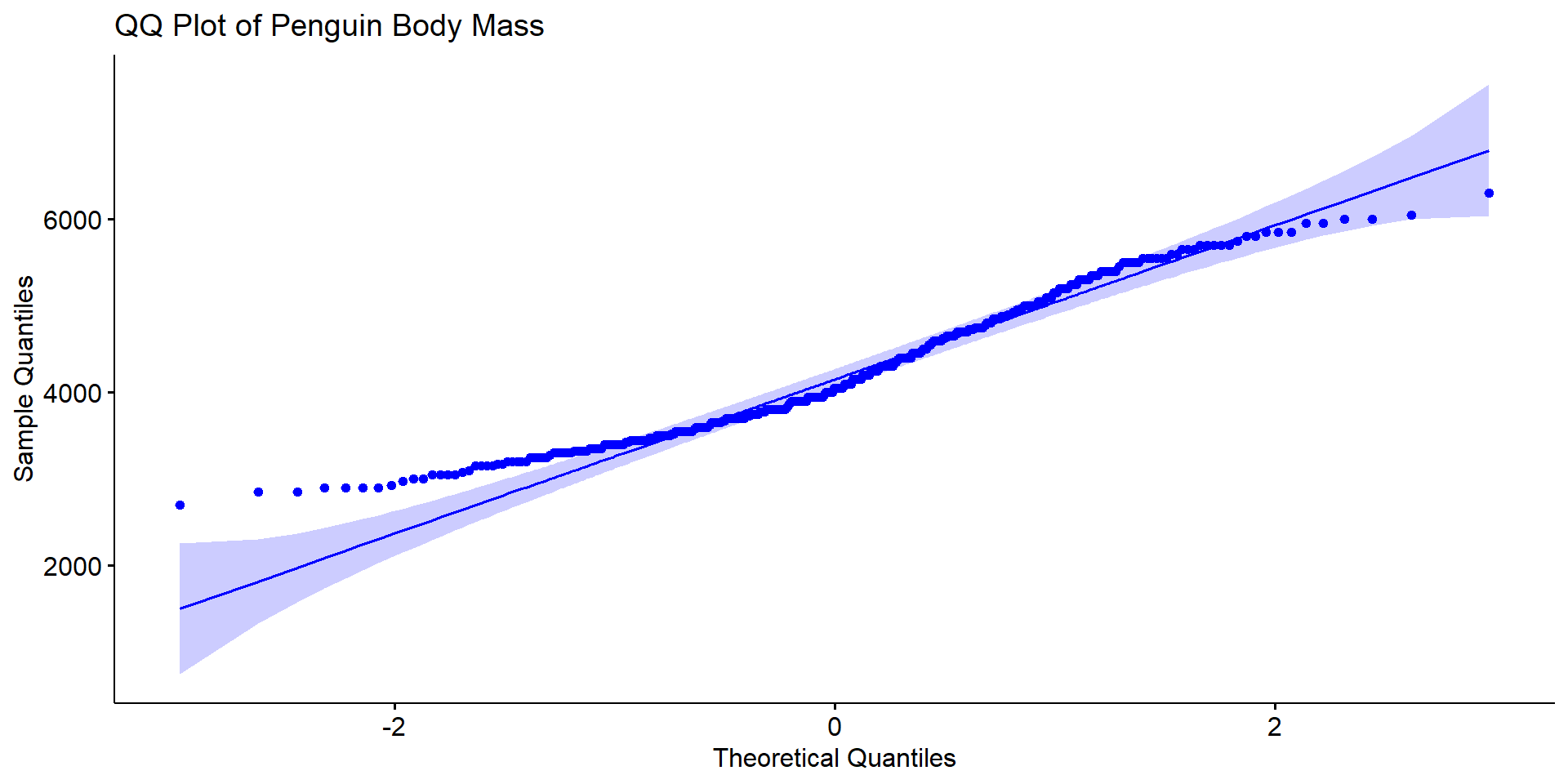

Again the ame conclusion, the variable body_mass_g does not look like it follows a normal distribution.

Shapiro-Wilk Test

Non-parametric test

Dependent variable	/
Independant variable	Quantitative

Asumption :

• The sample size is small to moderate (e.g. less than 2000 observations).

H0 : Null hypothesis

The sample comes from a normal distribution.

Example :

• The author tackle Shapiro-Wilk Nnormality test using R.

• The data will be created directly in R using the comand set.seed.

set.seed(946322) # generate random values
x1 = rnorm(100)
x2 = runif(100)

Question

Are the two variables normally distributed ?

We apply a shapiro test for the two variables.

shapiro.test(x1)

    Shapiro-Wilk normality test

data:  x1
W = 0.98862, p-value = 0.5548

• We get a p-value \(\simeq \ 0.55 \ \simeq \ 55 \% \ > \alpha\)

• Therefore we can accept H0.

• The sample X1 does look like it is normally distributed

shapiro.test(x2)

    Shapiro-Wilk normality test

data:  x2
W = 0.93307, p-value = 7.464e-05

• We get a p-value \(\simeq \ 7.5 \ 10^{-5} \ > \alpha\)

• Therefore we can reject H0.

• The sample X2 does NOT look like it is normally distributed

Kolmogorov-Smirnov Test

Non-parametric test

Dependent variable	/
Independant variable	Quantitative

Asumption :

• /

H0 : Null hypothesis

The sample comes from a normal distribution.

Example :

We create a variable Y :

Y <- c(8.43, 8.70, 11.27, 12.92, 13.05, 13.05, 13.17, 13.44, 13.89, 18.90)

• We are going to use the Kolmogorov-Smirnov test for an normal distribution.

• It is written like this :

ks.test(Y, "pnorm", mean = mean(Y), sd = sd(Y))

ks.test(Y,"pnorm", mean = mean(Y), sd = sd(Y))

    Asymptotic one-sample Kolmogorov-Smirnov test

data:  Y
D = 0.23999, p-value = 0.6122
alternative hypothesis: two-sided

• We get a p-value \(\simeq \ 0.61 \ \simeq \ 61 \% \ > \alpha\)

• Therefore we can accept H0.

• The sample Y does look like it is normally distributed

Tests for homogeneity of variances

There are two main tests.

Levene test

Non-parametric test

Dependent variable	Quantitative
Independant variable	Qualitative

Asumption :

• Independent observations

H0 : Null hypothesis

The variance among groups is equal.

Example :

We import the dataset titanic.csv

titanic.data = read.csv("data_raw/titanic.csv")

we load the required packages

library(car)
library(carData)

Question

In the dataset titanic, do the two groups deadand alive have the same variance ?

we perform our levene test

leveneTest(age ~ survive, data = titanic.data)

Levene's Test for Homogeneity of Variance (center = median)
       Df F value  Pr(>F)  
group   1  5.1144 0.02407 *
      631                  
---
Signif. codes:  0 '***' 0.001 '**' 0.01 '*' 0.05 '.' 0.1 ' ' 1

• We get a p-value \(\simeq \ 0.024 \ \simeq \ 2.4 \% \ < \alpha\)

• Therefore we can reject H0.

• The two groups do not have the same variance.

Bartlett test

Non-parametric test

Dependent variable	Quantitative
Independant variable	Qualitative

Asumption :

• It does not assume equal sample sizes across groups

H0 : Null hypothesis

The variance among groups is equal.

Example :

We use the same dataset titanic, but this time we change variable.

Question

In the dataset titanic, do the two groups femaleand male have the same variance ?

bartlett.test(age ~ sex, data = titanic.data)

    Bartlett test of homogeneity of variances

data:  age by sex
Bartlett's K-squared = 0.049888, df = 1, p-value = 0.8233

• We get a p-value \(\simeq \ 0.82 \ \simeq \ 8.2 \% \ > \alpha\)

• Therefore we can accept H0.

• The two groups have the same variance.

T-tests

There are different T-tests.

T-test for one sample

Parametric test

Dependent variable	Quantitative (continuous)
Independant variable	-

Asumptions :

• Normality : dependent variables should be normally distributed within each group

• Homogenity of variance

H0 : Null hypothesis

The sample mean is equal to the given reference value

Example :

We collect a sample of 10 birth weight of sheep.

weight = c(2, 1.5, 3, 2.5, 3.5, 4, 2.5, 2, 3, 1.5)

There are not outliers.

The null hypothesis H0 is : \(\mu = 3.5\), and we chose \(\alpha = 5 \%\).

t.test(weight, mu = 3.5, conf.level = 0.95)

    One Sample t-test

data:  weight
t = -3.6122, df = 9, p-value = 0.00564
alternative hypothesis: true mean is not equal to 3.5
95 percent confidence interval:
 1.955063 3.144937
sample estimates:
mean of x 
     2.55 

We get a p-value \(\simeq \ 0.006 \ \simeq \ 0.6 \% \ < \alpha\)

Therefore we can reject H0. The mean of the dataset if not equal to \(3.5\).

We can ask ourselves if the mean of the dataset is less or greater than \(3.5\).

The null hypothesis is just a bit different :

H0 : \(\mu < 3.5\)

t.test(weight, mu = 3.5, alternative = "greater", conf.level = 0.95)

    One Sample t-test

data:  weight
t = -3.6122, df = 9, p-value = 0.9972
alternative hypothesis: true mean is greater than 3.5
95 percent confidence interval:
 2.067899      Inf
sample estimates:
mean of x 
     2.55 

We get a p-value \(\simeq \ 0.997 \ \simeq \ 99.7 \% \ > \alpha\)

Therefore we can accep H0. The mean of the dataset if less than \(3.5\).

Independent t-test

Parametric test

Dependent variable	Quantitative (continuous)
Independant variable	Qualitatite (2 groups)

Asumptions :

• Normality : dependent variables should be normally distributed within each group
  \(\to\) if not met : Mann-Whitney test

• Homogenity of variance

• Does not assume equal sample sizes or equal variances between groups

• Assumes independent observations drawn from normally-distributed populations

• Robust against violations of normality when sample size is large

H0 : Null hypothesis

The groups have equal means.

Example :

We load the dataset bocks from the library GLMsData

library(GLMsData)
data(blocks)

we perform our t-test

t.test(Number ~ Shape, data = blocks)

    Welch Two Sample t-test

data:  Number by Shape
t = 7.4956, df = 77.669, p-value = 9.056e-11
alternative hypothesis: true difference in means between group Cube and group Cylinder is not equal to 0
95 percent confidence interval:
 1.96814 3.39186
sample estimates:
    mean in group Cube mean in group Cylinder 
                  8.16                   5.48 

• We get a p-value \(\simeq \ 9.05 \ 10^{-11} \ < \alpha\)

• Therefore we can reject H0.

• The two groups do NOT have the same mean.

Paired t-test

Parametric test

Dependent variable	Quantitative (continuous)
Independant variable	Time point 1 or 2 /condition

Asumptions :

• Normality : dependent variables should be normally distributed within each group
  \(\to\) if not met : Wilcoxon test

H0 : Null hypothesis

The groups have equal means.

Example :

# Weight of the mice before treatment
before <-c(200.1, 190.9, 192.7, 213, 241.4, 196.9, 172.2, 185.5, 205.2, 193.7)
# Weight of the mice after treatment
after <-c(392.9, 393.2, 345.1, 393, 434, 427.9, 422, 383.9, 392.3, 352.2)
# Create a data frame
my_data <- data.frame( 
                group = rep(c("before", "after"), each = 10),
                weight = c(before,  after)
                )
my_data

    group weight
1  before  200.1
2  before  190.9
3  before  192.7
4  before  213.0
5  before  241.4
6  before  196.9
7  before  172.2
8  before  185.5
9  before  205.2
10 before  193.7
11  after  392.9
12  after  393.2
13  after  345.1
14  after  393.0
15  after  434.0
16  after  427.9
17  after  422.0
18  after  383.9
19  after  392.3
20  after  352.2

we perfrom our paired t-test

t.test(before, after, paired = TRUE)

    Paired t-test

data:  before and after
t = -20.883, df = 9, p-value = 6.2e-09
alternative hypothesis: true mean difference is not equal to 0
95 percent confidence interval:
 -215.5581 -173.4219
sample estimates:
mean difference 
        -194.49 

• We get a p-value \(\simeq \ 6.2 \ 10^{-9} \ < \alpha\)

• Therefore we can reject H0.

• The two groups do NOT have the same mean.

Mann-Whitney test

Non-parametric equivalent to the independent t-test

Dependent variable	Ordinal/ Continuous
Independant variable	Qualitative

Asumption :

• independent samples

There are two types Mann-Whitney tests. If the distribution of scores for both groups have the same shape, the medians can be compared. If not, use the default test which compares the mean ranks

H0 : Null hypothesis

The median of the two groups are the same (if the distribution for both groups have the same shape), otherwise the mean ranks are the same.

Example :

movieRating = read.csv(file = "data_raw/95_Data_File.csv", header = TRUE, sep = ",")
head(movieRating)

  Male Female
1 6.35   5.90
2 6.54   6.28
3 6.11   5.76
4 6.97   6.66
5 6.78   6.71
6 5.83   5.58

wilcox.test(movieRating$Male,movieRating$Female, paired = FALSE)

    Wilcoxon rank sum test with continuity correction

data:  movieRating$Male and movieRating$Female
W = 255.5, p-value = 0.1368
alternative hypothesis: true location shift is not equal to 0

• We get a p-value \(\simeq \ 0.1368 \ > \alpha\)

• Therefore we can accept H0.

• The two groups do have the same median.

Wilcoxon test

Non-parametric equivalent to the paired t-test

Dependent variable	Ordinal/ Continuous
Independant variable	Time/ Condition

Asumption : /

H0 : Null hypothesis

The is no median difference between the paired observations.

Example :

aluLevels = read.csv(file = "data_raw/96_Data_File.csv", header = TRUE, sep = ",")
head(aluLevels)

          Clone August November
1         Primo   12.6     12.7
2      Raspalje    9.5     10.5
3     Hazendans   16.5     15.3
4     Hoogvorst   13.6     15.6
5 Fritzi Pauley   13.3     11.1
6  Balsam Spire    8.1     11.2

wilcox.test(aluLevels$August, aluLevels$November, paired = TRUE)

    Wilcoxon signed rank exact test

data:  aluLevels$August and aluLevels$November
V = 16, p-value = 0.03979
alternative hypothesis: true location shift is not equal to 0

• We get a p-value \(\simeq \ 0.039 \ = \ 0.39 \% \ > \alpha\)

• Therefore we can reject H0.

• The two groups do NOT have the same median.

ANOVA

ANalysis Of VAriance

One-way ANOVA

Parametric test

Dependent variable	Continuous
Independant variable	Qualitatives (3+ groups)

Asumptions :

• Residuals should be normally distributed

\(\to\) if not met : Kruskall-Wallis test

• Homogeneity of variance

H0 : Null hypothesis

The population means are all equal in the groups.

Example :

We load the required packages and the dataset chickwts

library(tidyverse)
head(chickwts)

  weight      feed
1    179 horsebean
2    160 horsebean
3    136 horsebean
4    227 horsebean
5    217 horsebean
6    168 horsebean

Question

Does the feed being used help explain the weights of chicken ?

We first look for homogeneity of variance.

library(car)
leveneTest(chickwts$weight ~ chickwts$feed)

Levene's Test for Homogeneity of Variance (center = median)
      Df F value Pr(>F)
group  5  0.7493 0.5896
      65               

• We get a p-value \(\simeq \ 0.59 \ = \ 59 \% \ > \alpha\)

• Therefore we can accept H0.

• The groups do have the same variance

model.ANOVA.OneWay = aov(chickwts$weight ~ chickwts$feed)

We need to check if the residuals are normally distributed

shapiro.test(model.ANOVA.OneWay$residuals)

    Shapiro-Wilk normality test

data:  model.ANOVA.OneWay$residuals
W = 0.98616, p-value = 0.6272

• We get a p-value \(\simeq \ 0.63 \ = \ 63 \% \ > \alpha\)

• Therefore we can accept H0.

• The residuals are normally distributed

Now we can analyse the ANOVA result :

summary(model.ANOVA.OneWay)

              Df Sum Sq Mean Sq F value   Pr(>F)    
chickwts$feed  5 231129   46226   15.37 5.94e-10 ***
Residuals     65 195556    3009                     
---
Signif. codes:  0 '***' 0.001 '**' 0.01 '*' 0.05 '.' 0.1 ' ' 1

• We get a p-value \(\simeq \ 5.94 . 10^{-10} \ < \alpha\)

• Therefore we can reject H0.

• The mean are not the same all the groups.

• The feed being used help explain the weights of chicken, but we cannot say how.

Two-way ANOVA

Parametric test

Dependent variable	Continuous
Independent variables	2 qualitative (2+ levels within each)

Asumptions :

• Residuals should be normally distributed

• Homogeneity of variance

H0 : Null hypothesis

• The means (by one factor) of the groups being compared are the same

• The means (by the other factor) of the groups being compared are the same

• There is no interaction between the two factors

The two-way ANOVA : extension of the one-way ANOVA that examines the influence of two different categorical independent variables on one continuous dependent variable.

The two-way ANOVA not only aims at assessing the main effect of each independent variable but also if there is any interaction between them.

Example :

head(ToothGrowth)

   len supp dose
1  4.2   VC  0.5
2 11.5   VC  0.5
3  7.3   VC  0.5
4  5.8   VC  0.5
5  6.4   VC  0.5
6 10.0   VC  0.5

We first look for homogeneity of variance.

library(car)
leveneTest(len ~ supp * factor(dose), data = ToothGrowth)

Levene's Test for Homogeneity of Variance (center = median)
      Df F value Pr(>F)
group  5  1.7086 0.1484
      54               

• We get a p-value \(\simeq \ 0.15 \ = \ 15 \% \ > \alpha\)

• Therefore we can accept H0.

• We have the homogeneity of variance.

model.ANOVA.TwoWay = aov(len ~ supp * factor(dose), data = ToothGrowth)

We need to check if the residuals are normally distributed

shapiro.test(model.ANOVA.TwoWay$residuals)

    Shapiro-Wilk normality test

data:  model.ANOVA.TwoWay$residuals
W = 0.98499, p-value = 0.6694

• We get a p-value \(\simeq \ 0.67 \ = \ 67 \% \ > \alpha\)

• Therefore we can accept H0.

• The residuals are normally distributed

Now we can analyse the Two-way ANOVA result :

                  Df Sum Sq Mean Sq F value   Pr(>F)    
supp               1  205.4   205.4  15.572 0.000231 ***
factor(dose)       2 2426.4  1213.2  92.000  < 2e-16 ***
supp:factor(dose)  2  108.3    54.2   4.107 0.021860 *  
Residuals         54  712.1    13.2                     
---
Signif. codes:  0 '***' 0.001 '**' 0.01 '*' 0.05 '.' 0.1 ' ' 1

• We get the a p-value \(\simeq \ 0.000231 \ < \alpha\)
  • Therefore we can reject the first part of the null hypothesis, which is : \(\to\) The means (by the factor supp) of the groups are NOT the same
• We get the a p-value \(\simeq \ 2 10^{-16} \ < \alpha\)
  • Therefore we can reject the second part of the null hypothesis, which is : \(\to\) The means (by the factor factor(dose)) of the groups are NOT the same
• We get the a p-value \(\simeq \ 0.022 \ < \alpha\)
  • Therefore we can reject the third part of the null hypothesis, which is : \(\to\) There IS an interaction between the two factors

Post hoc tests

In order to find out exactly which groups are different from each other, we must conduct a post hoc test.

• The Tukey test : compare all groups to each other

• The Dunnett test : compare with a reference group.

The Tukey test

Often follows a one-way ANOVA

Dependent variable	Continuous
Independant variable	Qualitatives (3+ groups)

Asumptions :

• the observations are independent,

• normality of distribution,

• homogeneity of variance.

H0 : Null hypothesis

The means of the tested groups are equal

Example 1 :

dietData = read.csv(file = "data_raw/90_Data_File.csv", header = TRUE, sep = ",")
head(dietData)

  Diet Weight.Week.1 Weight.Week.8 Weight.Loss
1    1            59            55           4
2    1            61            55           6
3    1            65            64           1
4    1            65            62           3
5    1            66            63           3
6    1            67            65           2

leveneTest(Weight.Loss ~ factor(Diet), data = dietData)

Levene's Test for Homogeneity of Variance (center = median)
      Df F value  Pr(>F)  
group  2  2.8097 0.06657 .
      75                  
---
Signif. codes:  0 '***' 0.001 '**' 0.01 '*' 0.05 '.' 0.1 ' ' 1

therefore we have homogeneity of variance

anova.tukey = aov(Weight.Loss ~ factor(Diet), data = dietData)
shapiro.test(anova.tukey$residuals)

    Shapiro-Wilk normality test

data:  anova.tukey$residuals
W = 0.98329, p-value = 0.3995

therefore we have normality

anova.tukey = aov(Weight.Loss ~ factor(Diet), data = dietData)
summary(anova.tukey)

             Df Sum Sq Mean Sq F value  Pr(>F)   
factor(Diet)  2   69.4    34.7   6.551 0.00239 **
Residuals    75  397.3     5.3                   
---
Signif. codes:  0 '***' 0.001 '**' 0.01 '*' 0.05 '.' 0.1 ' ' 1

therefore the means bewtween the groups are not the same

TukeyHSD(anova.tukey)

  Tukey multiple comparisons of means
    95% family-wise confidence level

Fit: aov(formula = Weight.Loss ~ factor(Diet), data = dietData)

$`factor(Diet)`
         diff        lwr      upr     p adj
2-1 0.3796296 -1.1643251 1.923584 0.8270005
3-1 2.1574074  0.6134526 3.701362 0.0036876
3-2 1.7777778  0.2799216 3.275634 0.0159151

only the comparison between groups 3 and 1 do have a p-value that indicate they might have different means

Example 2 :

We create our dataset

# response variable
size <- c(25,22,28,24,26,24,22,21,23,25,26,30,25,24,21,27,28,23,25,24,20,22,24,23,22,24,20,19,21,22)

# predictor variable
location <- as.factor(c(rep("ForestA",10), rep("ForestB",10), rep("ForestC",10)))

# dataframe
my.dataframe <- data.frame(size,location)
head(my.dataframe)

  size location
1   25  ForestA
2   22  ForestA
3   28  ForestA
4   24  ForestA
5   26  ForestA
6   24  ForestA

we check the homegeniety of variance

leveneTest(size ~ location, data = my.dataframe)

Levene's Test for Homogeneity of Variance (center = median)
      Df F value Pr(>F)
group  2  0.4919 0.6168
      27               

according to the p-value we have the homogeneity of variance

we check for the normality

shapiro.test(size[1-10])

    Shapiro-Wilk normality test

data:  size[1 - 10]
W = 0.97115, p-value = 0.5913

shapiro.test(size[11-20])

    Shapiro-Wilk normality test

data:  size[11 - 20]
W = 0.97115, p-value = 0.5913

shapiro.test(size[21-30])

    Shapiro-Wilk normality test

data:  size[21 - 30]
W = 0.97115, p-value = 0.5913

according to the p-values we have the normality

we perform our one-way ANOVA

my.ANOVA = aov(size ~ location, data = my.dataframe)
summary(my.ANOVA)

            Df Sum Sq Mean Sq F value  Pr(>F)   
location     2  66.47   33.23    7.11 0.00331 **
Residuals   27 126.20    4.67                   
---
Signif. codes:  0 '***' 0.001 '**' 0.01 '*' 0.05 '.' 0.1 ' ' 1

according to the p-value the means of the groups are not equal

we then perfrom our Tukey test

TukeyHSD(my.ANOVA)

  Tukey multiple comparisons of means
    95% family-wise confidence level

Fit: aov(formula = size ~ location, data = my.dataframe)

$location
                diff       lwr         upr     p adj
ForestB-ForestA  1.3 -1.097245  3.69724537 0.3835917
ForestC-ForestA -2.3 -4.697245  0.09724537 0.0619108
ForestC-ForestB -3.6 -5.997245 -1.20275463 0.0025530

• The output displays the results of all pairwise comparisons among the tested groups.

• The p-value for the comparison Forest B with Forest A is bigger than \(\alpha\).

  • Therefore their means are equal

• The p-value for the other comparisons are smaller than \(\alpha\).

  • Therefore their means are NOT equal

The Dunnett test

Often follows a one-way ANOVA

Dependent variable	Continuous
Independant variable	Qualitatives (3+ groups)

Asumptions :

• Groups being compared must be independent

H0 : Null hypothesis

The means of the control group and any other groups are the equal

Example :

We go back with our example from the tukey test.

We chose the forest A has a reference.

library(DescTools)
DunnettTest(x = my.dataframe$size, g = my.dataframe$location)

  Dunnett's test for comparing several treatments with a control :  
    95% family-wise confidence level

$ForestA
                diff     lwr.ci     upr.ci   pval    
ForestB-ForestA  1.3 -0.9562769  3.5562769 0.3160    
ForestC-ForestA -2.3 -4.5562769 -0.0437231 0.0453 *  

---
Signif. codes:  0 '***' 0.001 '**' 0.01 '*' 0.05 '.' 0.1 ' ' 1

• The p-value for the comparison Forest B with Forest A is bigger than \(\alpha\).
  • Therefore their means are equal
• The p-value for the comparison Forest C with Forest A is smaller than \(\alpha\).
  • Therefore their means are NOT equal

Kruskal-Wallis test

Non parametric equivalent to the one-way ANOVA

Dependent variable	Ordinal / Continuous
Independant variable	Qualitatives (3+ groups)

Asumptions :

• the observations are independent

• similar sample size

H0 : Null hypothesis

The mean ranks of the groups are the same.

Example :

sprayData <- read.csv(file = "data_raw/97_Data_File.csv",
    header = TRUE, sep = ",")
head(sprayData)

  Type.A Type.B Type.C Type.D Type.E Type.F
1     10     11      0      3      3     11
2      7     17      1      5      5      9
3     20     21      7     12      3     15
4     14     11      2      6      5     22
5     14     16      3      4      3     15
6     12     14      1      3      6     16

we perform our Kruskal-Wallis test

kwTest = kruskal.test(sprayData)
kwTest

    Kruskal-Wallis rank sum test

data:  sprayData
Kruskal-Wallis chi-squared = 54.691, df = 5, p-value = 1.511e-10

we get a very small p-value, therefore we can reject H0

Correlation-s tests

Non parametric equivalent to the one-way ANOVA

Dependent variable	Continuous
Independant variable	Continuous

Asumptions :

H0 : Null hypothesis

There is no linear relationship

Example :

We load the required packages

library("ggpubr")

Correlation coefficient can be computed using the functions cor or cor.test

we can choose between 3 methods :

• pearson
• kendall
• spearman

my_data <- mtcars
head(my_data)

                   mpg cyl disp  hp drat    wt  qsec vs am gear carb
Mazda RX4         21.0   6  160 110 3.90 2.620 16.46  0  1    4    4
Mazda RX4 Wag     21.0   6  160 110 3.90 2.875 17.02  0  1    4    4
Datsun 710        22.8   4  108  93 3.85 2.320 18.61  1  1    4    1
Hornet 4 Drive    21.4   6  258 110 3.08 3.215 19.44  1  0    3    1
Hornet Sportabout 18.7   8  360 175 3.15 3.440 17.02  0  0    3    2
Valiant           18.1   6  225 105 2.76 3.460 20.22  1  0    3    1

we plot our data

ggscatter(my_data, x = "mpg", y = "wt", 
          add = "reg.line", conf.int = TRUE, 
          cor.coef = TRUE, cor.method = "pearson",
          xlab = "Miles/(US) gallon", ylab = "Weight (1000 lbs)")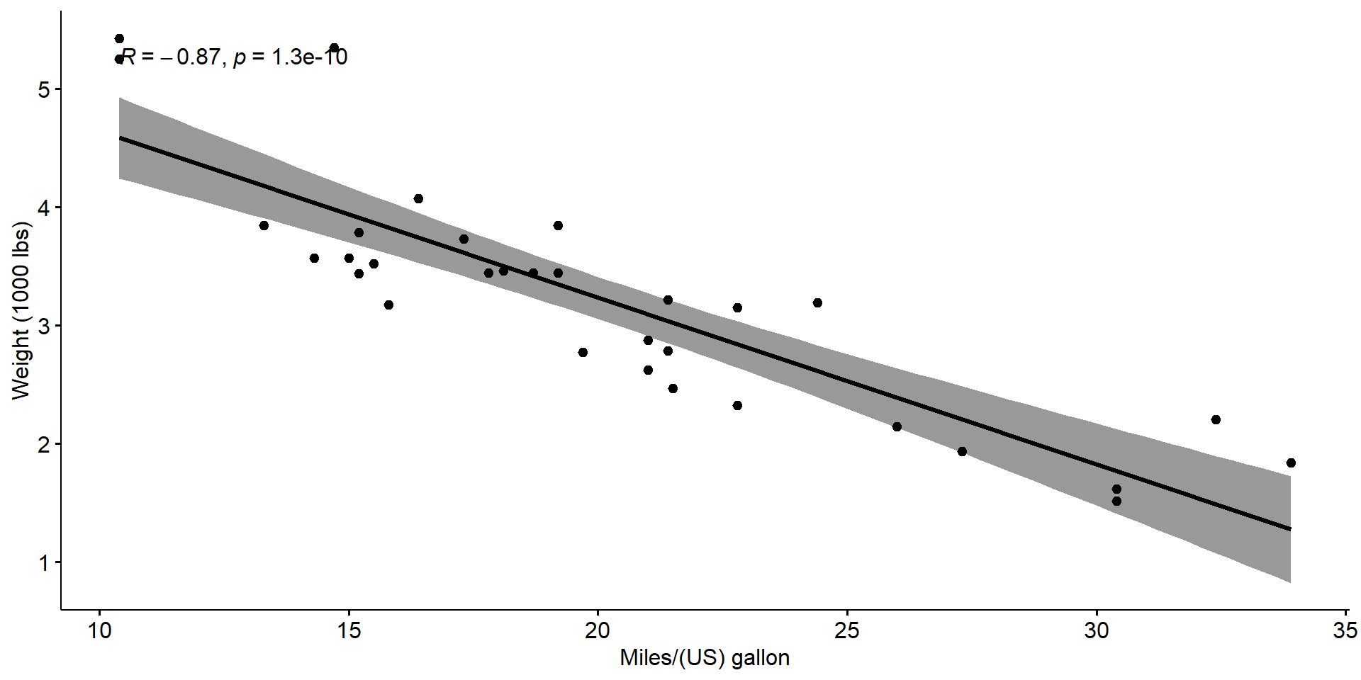

The Pearson correlation test

cor.test(my_data$wt, my_data$mpg, method = "pearson")

    Pearson's product-moment correlation

data:  my_data$wt and my_data$mpg
t = -9.559, df = 30, p-value = 1.294e-10
alternative hypothesis: true correlation is not equal to 0
95 percent confidence interval:
 -0.9338264 -0.7440872
sample estimates:
       cor 
-0.8676594 

• The p-value is less than \(\alpha\)
• We can conclude that wt and mpg are significantly correlated with a correlation coefficient of \(-0.87\)

Kendall rank correlation test

cor.test(my_data$wt, my_data$mpg,  method="kendall")

    Kendall's rank correlation tau

data:  my_data$wt and my_data$mpg
z = -5.7981, p-value = 6.706e-09
alternative hypothesis: true tau is not equal to 0
sample estimates:
       tau 
-0.7278321 

same conclusion as the Pearson correlation test

Spearman rank correlation coefficient

cor.test(my_data$wt, my_data$mpg,  method = "spearman")

    Spearman's rank correlation rho

data:  my_data$wt and my_data$mpg
S = 10292, p-value = 1.488e-11
alternative hypothesis: true rho is not equal to 0
sample estimates:
      rho 
-0.886422 

same conclusion as the previous correlation tests

Multiple Linear regression

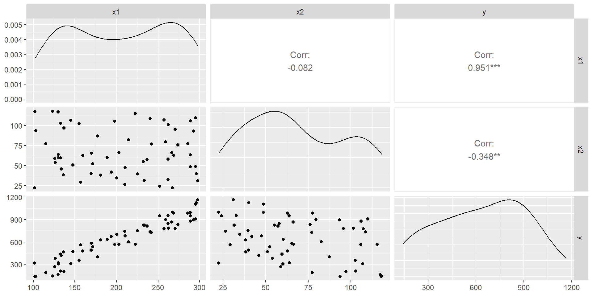
Few packages that are very useful to perform multiple linear regression

library(tidyverse)
library(GGally)
library(broom)

We “produce” data (FYI)

set.seed(2)
x1 = runif(60,100,300)
x2 = runif(60,20,120)
y = 20 + 4*x1 - 3*x2 + rnorm(60,0,40)
df = tibble(x1,x2,y)
new_x1 = seq(from = 120, to = 300, length.out = 20)
new_x2 = runif(20,30,110)
new_data = tibble(x1 = new_x1, x2 = new_x2)

our dataset is

head(df)

# A tibble: 6 × 3
     x1    x2     y
  <dbl> <dbl> <dbl>
1  137.  97.0  205.
2  240. 109.   737.
3  215.  82.5  603.
4  134.  46.0  423.
5  289. 106.   878.
6  289.  63.7  951.

Assumptions

Model of the form

\[y \sim \beta_0+\displaystyle\sum_{k=1}^p \beta_k x_k+\epsilon_i\]

• Assumes Linear relationship between \(y\) and \(x_1, x_2, \ldots, x_p\)
• Assumes the irreducible error (\(\epsilon_i\)) is normally distributed
• Assumes homoscedacisity, that is \(\epsilon_i\) does not depend on \(x_1, x_2, \ldots, x_p\)
• In this model, the variables \(x_i\) do not interact
• Always watch out for outliers !

A first look at the data

ggpairs(df)

The model

model = lm(y ~ x1 + x2, data = df)
summary(model)

Call:
lm(formula = y ~ x1 + x2, data = df)

Residuals:
    Min      1Q  Median      3Q     Max 
-72.286 -34.102  -2.892  30.163  87.738 

Coefficients:
             Estimate Std. Error t value Pr(>|t|)    
(Intercept) -35.39079   24.19773  -1.463    0.149    
x1            4.15232    0.08981  46.235   <2e-16 ***
x2           -2.66124    0.19657 -13.539   <2e-16 ***
---
Signif. codes:  0 '***' 0.001 '**' 0.01 '*' 0.05 '.' 0.1 ' ' 1

Residual standard error: 43.2 on 57 degrees of freedom
Multiple R-squared:  0.9772,    Adjusted R-squared:  0.9764 
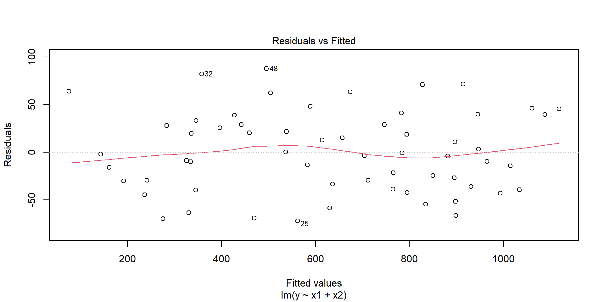
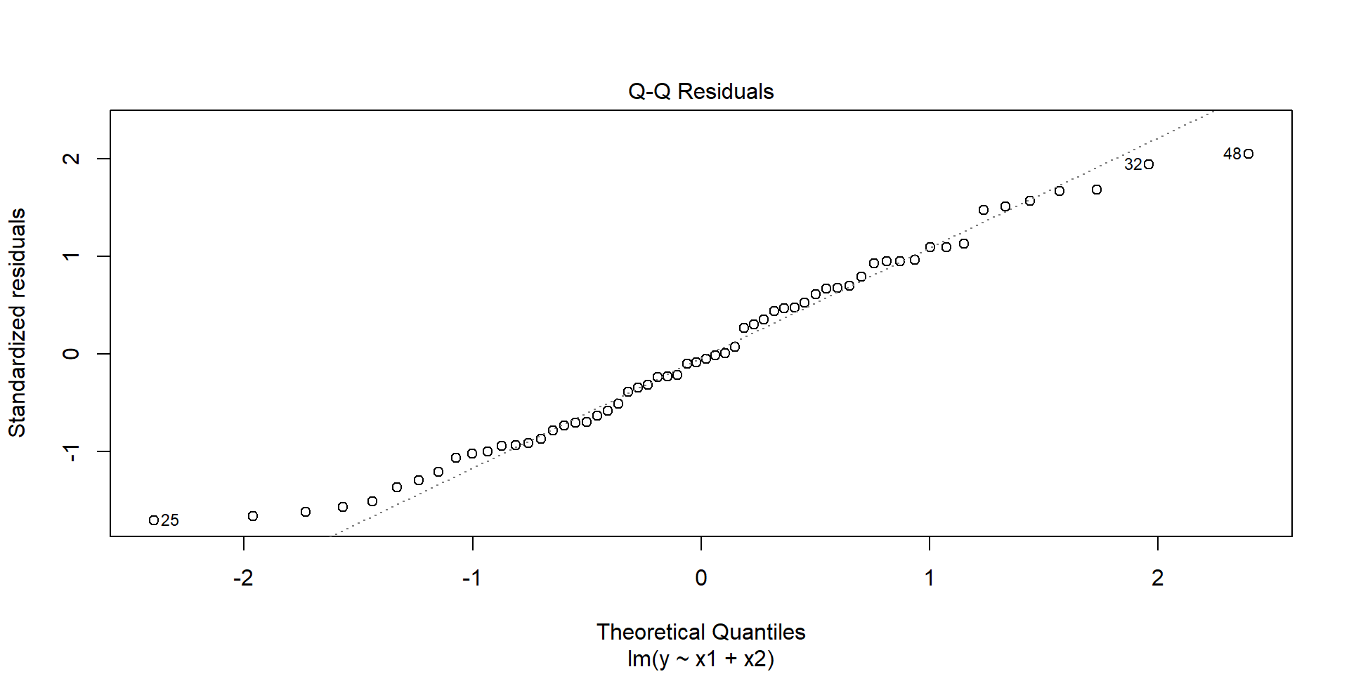
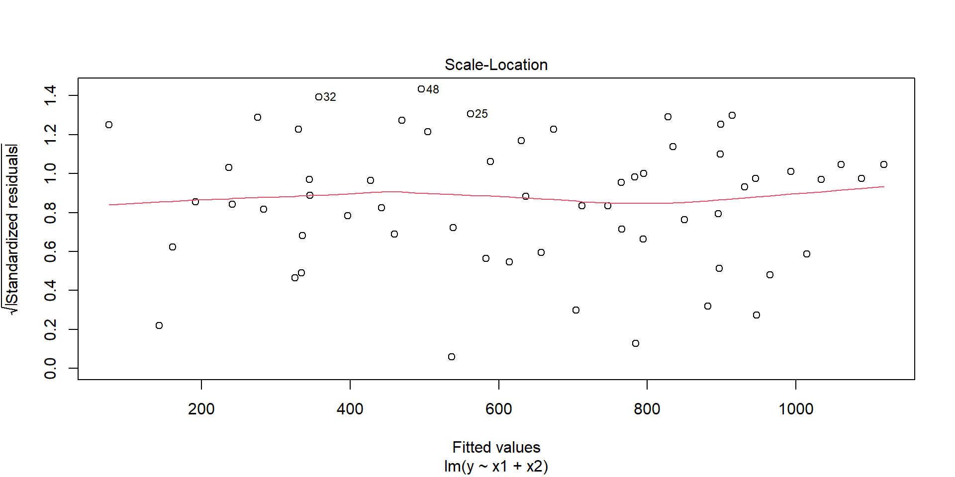
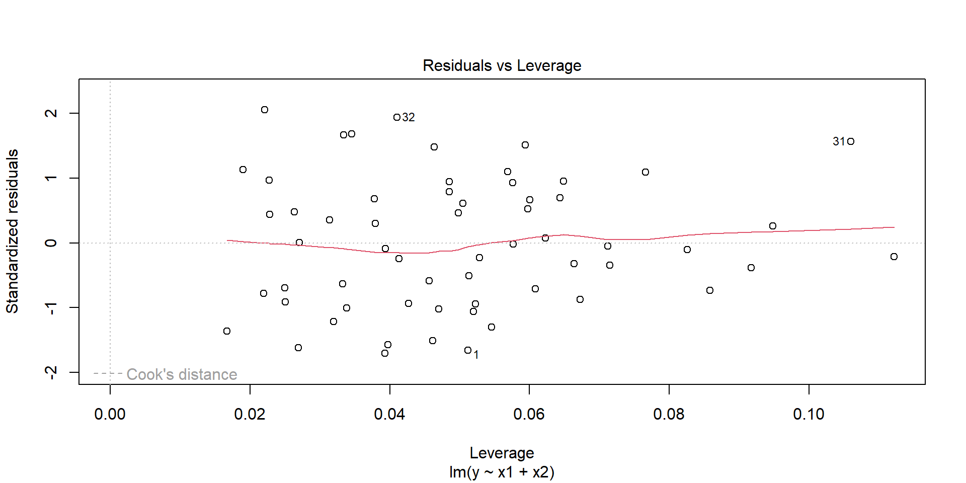
F-statistic:  1220 on 2 and 57 DF,  p-value: < 2.2e-16

Few graphs to undersand the model

plot(model)

Predictions

new_data

# A tibble: 20 × 2
      x1    x2
   <dbl> <dbl>
 1  120  101. 
 2  129.  54.1
 3  139.  74.4
 4  148.  90.4
 5  158. 107. 
 6  167. 106. 
 7  177.  56.7
 8  186.  71.3
 9  196.  41.9
10  205.  58.5
11  215.  86.4
12  224.  36.4
13  234.  50.1
14  243.  34.1
15  253.  89.1
16  262.  31.1
17  272.  33.4
18  281.  52.5
19  291.  33.3
20  300   80.6

\(\to\) We want to “predict” the y according to these x1 and x2

fit = predict(model,new_data)
new_data$predict = fit
new_data

# A tibble: 20 × 3
      x1    x2 predict
   <dbl> <dbl>   <dbl>
 1  120  101.     193.
 2  129.  54.1    358.
 3  139.  74.4    344.
 4  148.  90.4    340.
 5  158. 107.     337.
 6  167. 106.     377.
 7  177.  56.7    548.
 8  186.  71.3    548.
 9  196.  41.9    666.
10  205.  58.5    661.
11  215.  86.4    626.
12  224.  36.4    799.
13  234.  50.1    802.
14  243.  34.1    883.
15  253.  89.1    777.
16  262.  31.1    970.
17  272.  33.4   1003.
18  281.  52.5    992.
19  291.  33.3   1082.
20  300   80.6    996.

Factor analysis

Principal Component Analysis

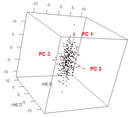
Problem

We are working with a problem with way too many dimensions

Goals

1. Dimension reduction to a few dimensions while explaining most of the variance

2. Find one-dimensional index that separates objects best

Intuition

Note

Find low-dimensional projection with largest spread

• Dimension reduction : Only keep coordinate of first (few) Principal Component (PC)

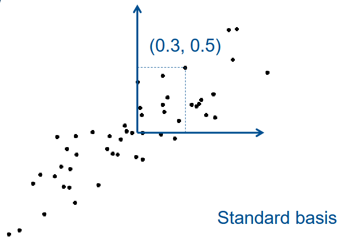
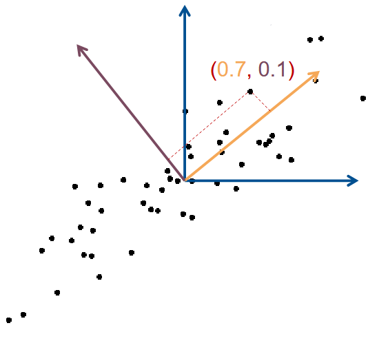
• Rotated basis :

  • Vector 1 : Largest variance (1st PC)
  • Vector 2 : Perpendicular (2nd PC)

	x1	x2
Std. Basis	0.3	0.5
PC Basis	0.7	0.1
After Dim. Reduc.	0.7	-

Orthogonal directions

• PC 1 is the direction with largest variance

• PC 2 is :

  • perpendicular to PC 1
  • again largest variance

• PC 3 is :

  • perpendicular to PC 1, PC 2
  • again largest variance

• …

Which kinds of data ?

PCA applies to data tables where : - rows are considered as individuals - and columns as quantitative variables

Example :

The data :

	\(P\) \(\left(\text{cm}\right)\)	\(T_{\text{max}}\) \(\left(^\circ C\right)\)	\(T_{\text{min}}\) \(\left(^\circ C\right)\)
Ajaccio	12,04	23,7	5,9
Brest	17,18	15,5	-1,8
Dunkerque	11,83	13,1	2,8
Nancy	6,23	13,5	-2,4
Nice	16,99	21,1	7,2
Toulouse	3,87	20,3	-0,9
\(\mu\)	11,36	17,87	1,8
\(\sigma\)	4,98	4,04	3,76

We can center and reduce this dataset using the relation

\[x_{i k}=\frac{x_{i k}-\overline{X_k}}{\sigma_k}\] we get

	\(P\) \(\left(\text{cm}\right)\)	\(T_{\text{max}}\) \(\left(^\circ C\right)\)	\(T_{\text{min}}\) \(\left(^\circ C\right)\)
Ajaccio	0,14	1,44	1,09
Brest	1,17	-0,59	-0,96
Dunkerque	0,10	-1,18	0,27
Nancy	-1,03	-1,08	-1,12
Nice	1,13	0,80	1,44
Toulouse	-1,50	0,60	-0,72

We call it \(X_{cr}\)

\[X_{cr} =\left[\begin{array}{rrr}0,14 & 1,44 & 1,09 \\ 1,17 & -0,59 & -0,96 \\ 0,10 & -1,18 & 0,27 \\ -1,03 & -1,08 & -1,12 \\ 1,13 & 0,80 & 1,44 \\ -1,50 & 0,60 & -0,72\end{array}\right]\]

we can define the correlation Matrix

	\(P\)	\(T_{\text{max}}\)	\(T_{\text{min}}\)
\(P\)	1	\(r\left(P, T_{\text{max} }\right)\)	\(r\left(P, T_{\text{min} }\right)\)
\(T_{\text{max} }\)	\(r\left(T_{\text{max} }, P\right)\)	1	\(r\left(T_{\text{max} }, T_{\text{min} }\right)\)
\(T_{\text{min} }\)	\(r\left(T_{\text{min} }, P\right)\)	\(r\left(T_{\text{min} }, T_{\text{max} }\right)\)	1

where \(r\) are the correlations between 2 variables

\[r\left(P, T_{\text{max} }\right) = r\left(T_{\text{max} }, P\right)\]

\[C = \frac{1}{N} \ X_{cr}^T \ X_{cr}\] where here \(N=6\).

	\(P\)	\(T_{\text{max} }\)	\(T_{\text{min} }\)
\(P\)	1	0,09	0,49
\(T_{\text{max} }\)	0,09	1	0,62
\(T_{\text{min} }\)	0,49	0,62	1

We write

\[C = \begin{pmatrix} 1 & 0.09 & 0.49 \\ 0.09 & 1 & 0.62 \\ 0.49 & 0.62 & 1 \end{pmatrix}\]

we then look for eigenvalues and eigenvectors. We find

• \(\lambda_1 = 1,83\quad\) with \(\quad v_1=\begin{pmatrix} 0.46 \\ 0.56 \\ 0.69 \end{pmatrix}\)
• \(\lambda_2 = 0.92\quad\) with \(\quad v_2=\begin{pmatrix} 0.79 \\ -0.61 \\ -0.03 \end{pmatrix}\)
• \(\lambda_3 = 0.25\quad\) with \(\quad v_3=\begin{pmatrix} 0.41 \\ 0.56 \\ -0.72 \end{pmatrix}\)

The Inertia (generalized variance) is given by

\[ \mbox{Total inertia} = \sum \mbox{eigenvalues} \ = 3 \]

	Eigenvalue	Inertia (%)	Inertia Cumul. (%)
\(\lambda_1\)	1,83	61,17	61,17
\(\lambda_2\)	0,92	30,51	91,68
\(\lambda_3\)	0,25	8,32	100,00

Principal components

In order to get the principal components we compute

\[F_1 = X_{cr} v_1 \quad \mbox{ and } \quad F_2 = X_{cr} v_2\]

We get

\[F_1 = \begin{pmatrix} 1,63 \\ -0,45 \\ -0,43 \\ -1,85 \\ 1,96 \\ -0,85 \end{pmatrix} \quad \mbox{ and } \quad F_2 = \begin{pmatrix}-0,81 \\ 1,31 \\ 0,79 \\ -0,12 \\ 0,37 \\ -1,54\end{pmatrix}\] These two vectors form a plane which have \(~92 \%\) of the (generalized) variance. We can represent the indivuals and the variables in this plane with the coorelation circle

	\(\mathrm{F}_1\)	\(\mathrm{F}_2\)
Ajaccio	1,63	-0,81
Brest	-0,45	1,31
Dunkerque	-0,43	0,79
Nancy	-1,85	-0,12
Nice	1,96	0,37
Toulouse	-0,85	-1,54
\(\mu\)	0	0
\(\sigma^2\)	1,83	0,92

\(r(P,F_1) = \mbox{First coordinate of } v_1 \times \sqrt{\lambda_1} = 0.62\)

	\(F_1\)	\(F_2\)
\(P\)	\(0,62\)	\(0,76\)
\(T_{\text{max} }\)	\(0,76\)	\(-0,59\)
\(T_{\min }\)	0,93	\(-0,03\)

Time to look at an example

First example of PCA

data("iris")
head(iris)

  Sepal.Length Sepal.Width Petal.Length Petal.Width Species
1          5.1         3.5          1.4         0.2  setosa
2          4.9         3.0          1.4         0.2  setosa
3          4.7         3.2          1.3         0.2  setosa
4          4.6         3.1          1.5         0.2  setosa
5          5.0         3.6          1.4         0.2  setosa
6          5.4         3.9          1.7         0.4  setosa

we modify a bit the data for this example :

set.seed(111)
ind <- sample(2, nrow(iris),
              replace = TRUE,
              prob = c(0.8, 0.2))
training <- iris[ind==1,]
testing <- iris[ind==2,]

let’s do the principal component analysis

pc <- prcomp(training[,-5],
             center = TRUE,
            scale. = TRUE)
attributes(pc)

$names
[1] "sdev"     "rotation" "center"   "scale"    "x"       

$class
[1] "prcomp"

print(pc)

Standard deviations (1, .., p=4):
[1] 1.7173318 0.9403519 0.3843232 0.1371332

Rotation (n x k) = (4 x 4):
                    PC1         PC2        PC3        PC4
Sepal.Length  0.5147163 -0.39817685  0.7242679  0.2279438
Sepal.Width  -0.2926048 -0.91328503 -0.2557463 -0.1220110
Petal.Length  0.5772530 -0.02932037 -0.1755427 -0.7969342
Petal.Width   0.5623421 -0.08065952 -0.6158040  0.5459403

we have the principal components

For making biplot need devtools package.

library(ggbiplot)
g <- ggbiplot(pc,
              obs.scale = 1,
              var.scale = 1,
              groups = training$Species,
              ellipse = TRUE,
              circle = TRUE,
              ellipse.prob = 0.68)
g <- g + scale_color_discrete(name = '')
g <- g + theme(legend.direction = 'horizontal',
               legend.position = 'top')
g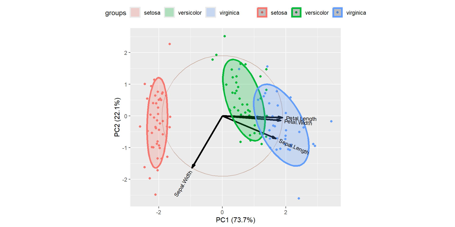

PC1 explains about 73.7% and PC2 explained about 22.1% of variability.

Arrows are closer to each other indicates the high correlation.

For example correlation between Sepal Width vs other variables is weakly correlated.

Another way interpreting the plot is PC1 is positively correlated with the variables Petal Length, Petal Width, and Sepal Length, and PC1 is negatively correlated with Sepal Width.

PC2 is highly negatively correlated with Sepal Width.

Bi plot is an important tool in PCA to understand what is going on in the dataset.

Hierarchical clustering analysis

cf. your notes

First example of HCA

we load the required packages

library(ggplot2)
library(NbClust)
library(cluster) 
library(factoextra)

we load the data

data.cluster = read.csv(file = "data_raw/food-bank.csv",header = FALSE, sep = ",")
head(data.cluster)

       V1      V2
1 0.04769 0.21150
2 0.05249 0.02238
3 0.10669 0.08343
4 0.14947 0.10921
5 0.18864 0.04716
6 0.19818 0.15651

we plot the data in the basis (V1,V2)

ggplot(data.cluster)+geom_point(aes(x=V1,y=V2))

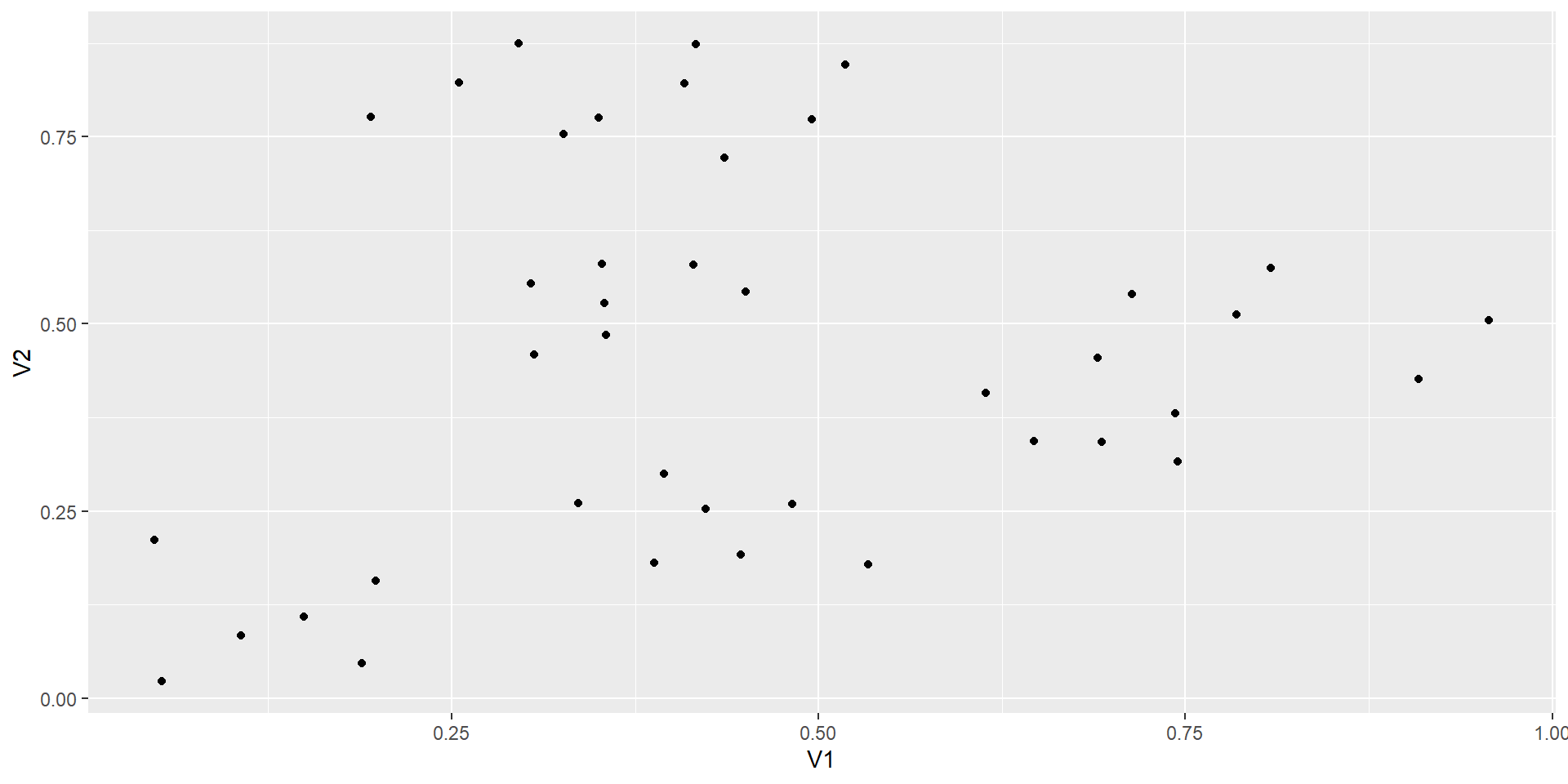
we want to cluster the coordinates

we define the euclidean distance (it is a choice that makes sense in this case)

dd <- dist(scale(data.cluster[,1:2]), method = "euclidean")

with ddwe get the distance between every coodinates.

we can now regroup the coordinates using the ward.D2 method

# hierarchical clustering
hc <- hclust(dd, method = "ward.D2")
plot(hc,hang = -1,labels = FALSE)

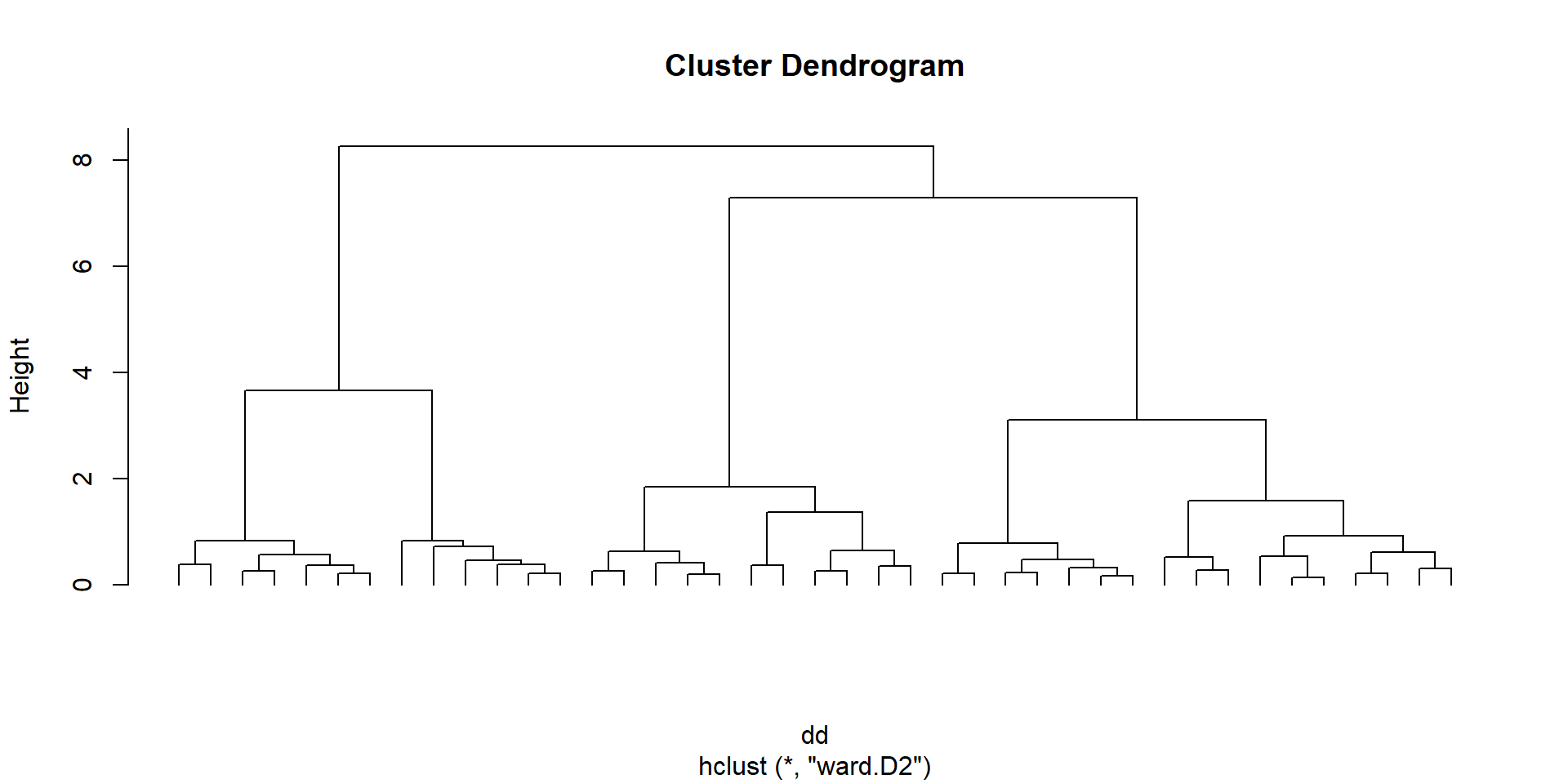
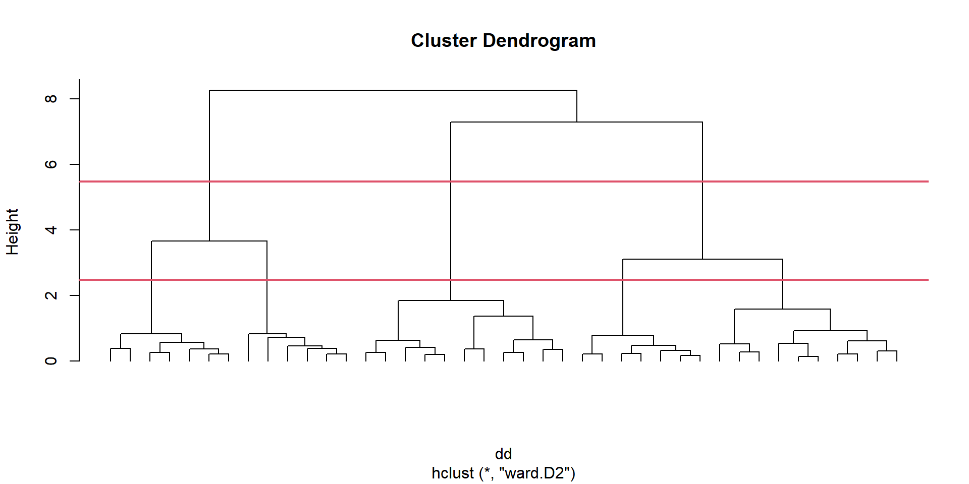
• the graph with all the clusters is called a dendogram

• we have to decide where to cut this dendogram to have groups to work with

• we plot the heights of this cluster analysis

barplot(diff(hc$height))

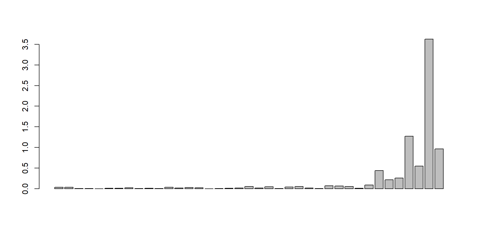
we will cut the tree at a given number of clusters and obtain the associated cluster for each observation

plot(hc,hang = -1,labels = F)
abline(h=mean(hc$height[38:39]),col=2,lwd=2)
abline(h=mean(hc$height[36:37]),col=2,lwd=2)