Trèfle de Habenicht

---

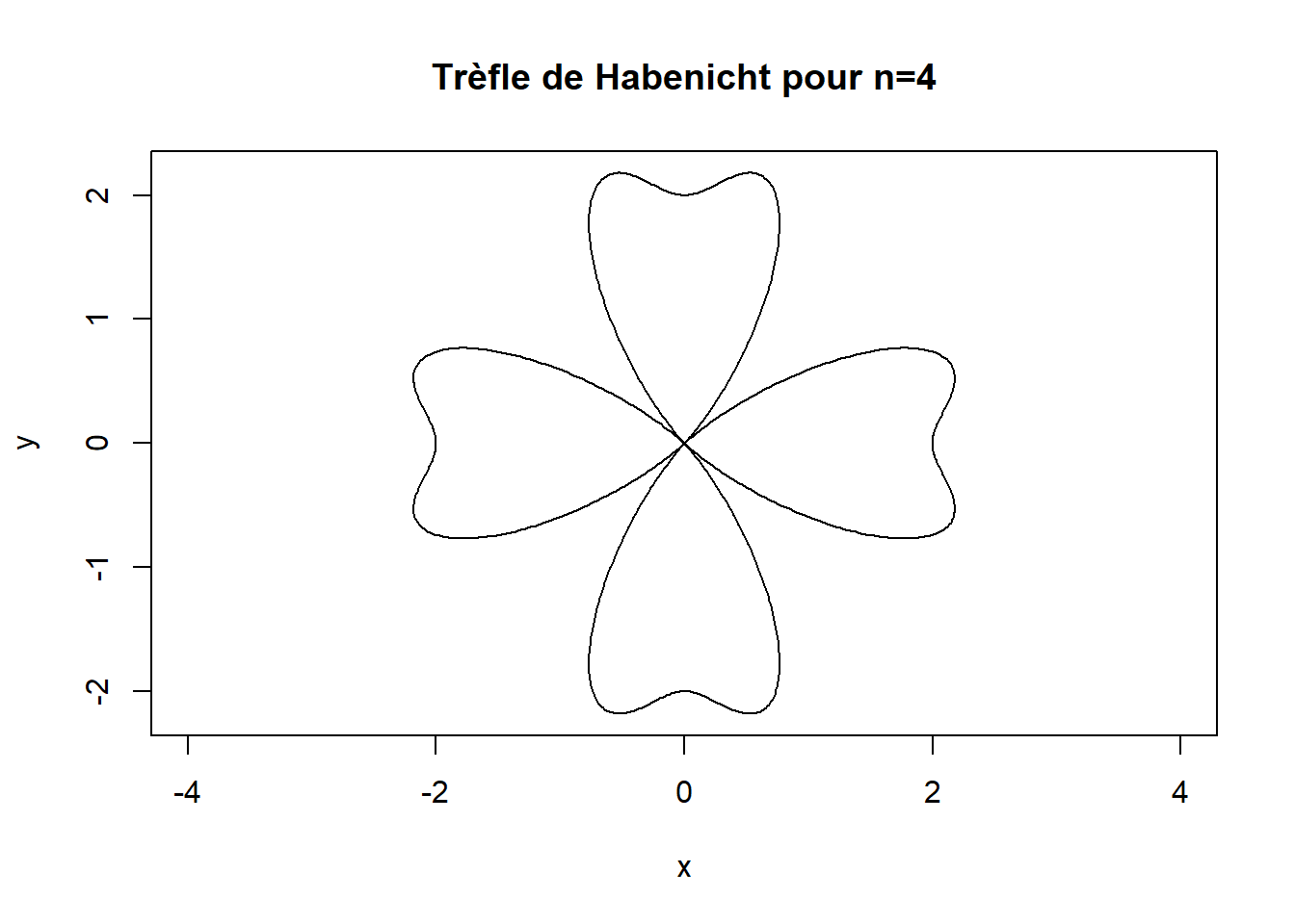
Nous allons étudier le Trèfle de Habenicht définie par son équation polaire. Son équation polaire est \[\rho = 1 +\cos\left(n\theta\right) + \sin^2\left(n\theta\right)\] L’objectif est de tracer le Trèfle de Habenicht pour \(n = 3\) ou \(n = 4\), selon la chance espérée ! 🍀

Nous choisirons ici de travailler dans le cas “chanceux” 🍀 \(n=4\)❗️

Domaine d’étude

L’équation polaire est alors \[\rho = 1 +\cos\left(4\theta\right) + \sin^2\left(4\theta\right)\] Le domaine de définition est \[D_1 = \mathbb{R}\]

On remarque que \(\rho\) est périodique de période \(\dfrac{\pi}{2}\). En effet on peut écire

\[\begin{align*} \rho\left(\theta+\frac{\pi}{2}\right) &= 1 +\cos\left(4\theta + 2\pi\right) + \sin^2\left(4\theta + 2\pi\right) \\ &= 1 +\cos\left(4\theta\right) + \sin^2\left(4\theta\right) \\ &=\rho\left(\theta\right) \end{align*}\]

On peut alors limiter l’étude à un intervalle d’amplitude \(\dfrac{\pi}{2}\). On completera par autant de rotations qu’il faut pour retomber sur l’arc de courbe initial.

\[D_2 = \left[-\dfrac{\pi}{4},\dfrac{\pi}{4}\right]\] De plus on remarque que \(\rho\) est paire en \(\theta\), c’est à dire \[\rho\left(-\theta\right)=\rho\left(\theta\right)\] Donc les point \(M_1\left(\rho,\theta\right)\) et \(M_2\left(\rho,-\theta\right)\) sont symétriques par rapport à l’axe des abscisses. On peut donc limiter l’étude à \[D_3 = \left[0,\dfrac{\pi}{4}\right]\]

Calcul de \(\rho^\prime\)

On calcule la dérivée de \(\rho\). On a

\[\rho\left(\theta\right)^\prime = 4\sin(4\theta) \left(2 \cos(4\theta) - 1 \right)\]

Donc

\[\rho\left(\theta\right)^\prime = 0 \ \Longleftrightarrow \theta = \left\{ 0 , \frac{\pi}{12} , \frac{\pi}{4} \right\}\]

Etude des variations de \(\rho\)

Etude des tangentes à la courbe

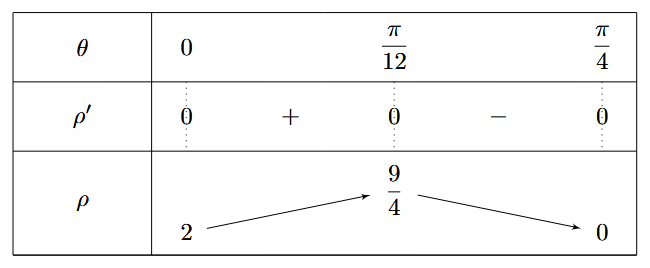
On peut à présent étudier les tangentes particulière en \[\theta = \left\{ 0, \ \dfrac{\pi}{12}, \ \dfrac{\pi}{4}\right\}\]

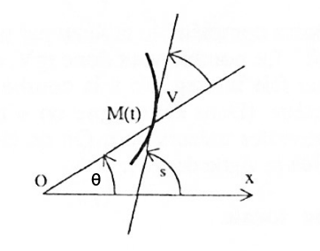
C’est langle \(V\) (défini sur la figure ci-dessus) qui nous interesse. On a

\[\tan\left(V\right) = \frac{\rho}{\rho^\prime}\]

Donc

\[\lim_{\theta \to 0 } \tan\left(V\right) = + \infty\]

\[\lim_{\theta \to \frac{\pi}{12} } \tan\left(V\right) = + \infty\]

\[\lim_{\theta \to \frac{\pi}{4}} \tan\left(V\right) = 0\]

On a donc

	\(\rho\)	\(\theta\)	\(V\)
\(M_0\)	\(2\)	\(0\)	\(\frac{\pi}{2}\)
\(M_1\)	\(\frac{9}{4}\)	\(\frac{\pi}{12}\)	\(\frac{\pi}{12}\)
\(M_2\)	\(0\)	\(\frac{\pi}{4}\)	\(0\)

Tracé

On trace cette courbe avec R.

theta <- seq(0, 2*pi, length.out = 1000)

rho <- 1 + cos(4*theta) + sin(4*theta)^2

x <- rho * cos(theta)
y <- rho * sin(theta)

plot(x, y, 
     type="l", 
     asp=1,  
     main="Trèfle de Habenicht pour n=4")

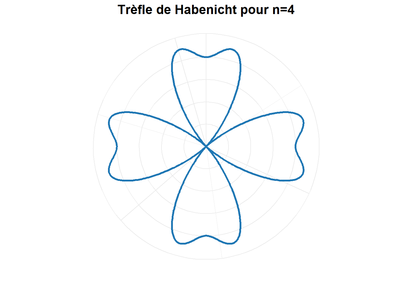
library(ggplot2)

theta <- seq(0, 2*pi, length.out = 1000)

rho <- 1 + cos(4*theta) + sin(4*theta)^2

data <- data.frame(theta = theta, rho = rho)

ggplot(data, aes(x = theta, y = rho)) +
  geom_path(color = "#1f77b4", size = 1.2) +
  coord_polar(theta = "x") +
  theme_minimal() +
  labs(title = "Trèfle de Habenicht pour n=4", x = "", y = "") +
  theme(
    plot.title = element_text(hjust = 0.5, size = 16, face = "bold"),
    axis.text = element_blank(),
    axis.ticks = element_blank()
  )